HW4: Finding the same cell type in Eevee data

What’s changed?
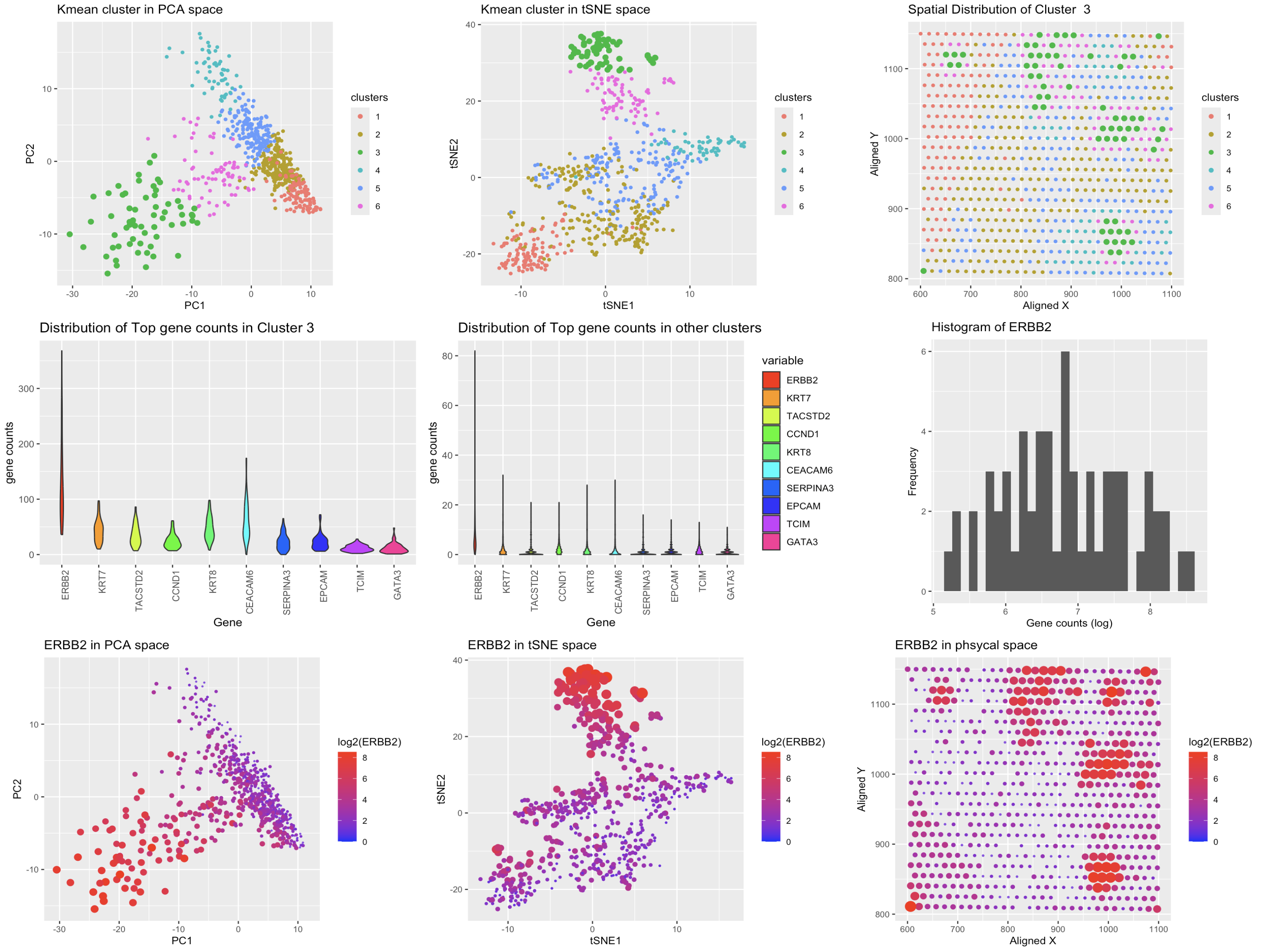
- The data pipeline had to be modified to accomodate the new data structure. Since Eevee data contained much more variables, that are not present in the Pikachu data, the data comparison required some adjustments. I decided to look at the features that are common between the two datasets, and also made sure check that the genes that were highly expressed in the cluster chosen in th Pikachu data were also present in the Eevee data, which narrowed down the Eevee data to ~300 genes.
- To reassure the clustering was approoriate, I added total-withiness test to check the optimal number of clusters.
- Also, in order to check for the similarity of the cluster found in the Pikachu data, I performed a t-test and wilcox test to compare the gene expression of the cluster of interest with the rest of the data, for each top 10 genes we identified in the previous HW. The results showed that the cluster of interest had a significant difference in gene expression compared to the rest of the data.
| Gene | t-test p-value | Wilcox p-value |
|-----------|----------------------|----------------------|
| ERBB2 | 4.978006e-53 | 2.026579e-38 |
| KRT7 | 7.900056e-61 | 2.925715e-40 |
| TACSTD2 | 7.002640e-53 | 5.723142e-44 |
| CCND1 | 3.653192e-46 | 5.704738e-39 |
| KRT8 | 1.007252e-63 | 1.309750e-40 |
| CEACAM6 | 1.372688e-40 | 1.226277e-39 |
| SERPINA3 | 2.732420e-34 | 1.028702e-41 |
| EPCAM | 7.404049e-47 | 2.092335e-42 |
| TCIM | 4.007187e-39 | 6.128568e-38 |
| GATA3 | 7.608228e-32 | 3.918908e-41 |
- As the table shows, the p-values for both tests are very low, which indicates that the cluster of interest has a significant difference in gene expression compared to the rest of the data as it was the case in the cluster found in the Pikachu data.
1
2
3
4
5
6
7
8
9
10
11
12
13
14
15
16
17
18
19
20
21
22
23
24
25
26
27
28
29
30
31
32
33
34
35
36
37
38
39
40
41
42
43
44
45
46
47
48
49
50
51
52
53
54
55
56
57
58
59
60
61
62
63
64
65
66
67
68
69
70
71
72
73
74
75
76
77
78
79
80
81
82
83
84
85
86
87
88
89
90
91
92
93
94
95
96
97
98
99
100
101
102
103
104
105
106
107
108
109
110
111
112
113
114
115
116
117
118
119
120
121
122
123
124
125
126
127
128
129
130
131
132
133
134
135
136
137
138
139
140
141
142
143
144
145
146
147
148
149
150
151
152
153
154
155
156
157
158
159
160
161
162
163
164
165
166
167
168
library(gridExtra)
library(ggplot2)
library(stats)
library(reshape2)
library(patchwork)
library(glue)
library(rlang)
library(Rtsne)
library(MASS)
library(ggpubr)
set.seed(42)

# please change the path to the data file
data_E <- read.csv("../data/eevee.csv.gz")
data_P <- read.csv("../data/pikachu.csv.gz")

# Picachu data
gexp_P <- data_P[, 7:ncol(data_P)]
# log transform the gexp data
log_gexp_P <- log2(gexp_P+1)

# Eevee data
gexp_E <- data_E[, 5:ncol(data_E)]
# find zero columns and remove them
zero_cols_E <- colnames(gexp_E)[colSums(gexp_E) == 0]
gexp_E <- gexp_E[, !(colnames(gexp_E) %in% zero_cols)]

# Find genes that are present in both Picachu and Eevee data
topgenes_P <- names(sort(colSums(gexp_P), decreasing=TRUE))
topgenes_E <- names(sort(colSums(gexp_E), decreasing=TRUE))
common_genes <- intersect(topgenes_P, topgenes_E)
print(glue("found {length(common_genes)} common genes in both datasets"))

# slice out the common genes to narrow down the data
common_gexp_P <- gexp_P[, common_genes]
common_gexp_E <- gexp_E[, common_genes]

# log transform the gexp data
log_gexp_E <- log2(common_gexp_E+1)

# PCA
pca_E <- prcomp(log_gexp_E, scale=TRUE)

# tSNE
emb_E <- Rtsne(log_gexp_E, dims=3, pca = TRUE, perplexity=30, verbose=FALSE)
# change the column name
colnames(emb_E$Y) <- c("tSNE1", "tSNE2", "tSNE3")

# perform kmeans clustering
df_E <- cbind(data_E, pca_E$x, emb_E$Y)

# Kmeans clustering
## determine the number of clusters
total_withinss <- c()
for (i in 1:10){
  kmeans <- kmeans(log_gexp_E, centers=i)
  total_withinss <- c(total_withinss, kmeans$tot.withinss)
}
# plot the total withinss with the number of clusters
tmp <- data.frame(
  clusters = 1:10,
  total_withinss = total_withinss
)

# Plot
e0 <- ggplot(tmp, aes(x = clusters, y = total_withinss)) +
      geom_line() +  # Line plot
      geom_point() +
      labs(
        title = "Total withinss vs Number of Clusters",
        x = "Number of Clusters",
        y = "Total Withinss"
      ) +
      theme_minimal()
e0

# From the scree plot, we choose cluster numbers
k=6
# k-means clustering on the original data
set.seed(42)
kmeans_orig <- kmeans(log_gexp_E, centers=k)
df_E$clusters <- as.factor(kmeans_orig$cluster)
# pick a cluster of interest
c <- 3
# create a vector of size, where 1 if the cluster is the cluster of interest, 0 otherwise
sizes <- ifelse(df_E$clusters == c, 2, 1)

# A panel visualizing your one cluster of interest in reduced dimensional space (PCA, tSNE, etc)
e1 <- ggplot(df_E) + geom_point(aes(x=PC1, y=PC2, color=clusters), size=sizes) + ggtitle("Kmean cluster in PCA space") + theme(aspect.ratio=1.0) + xlab("PC1") + ylab("PC2") + theme(text = element_text(size=10)) #+ theme(legend.position="none")
e1

# visulaize the clusters on tSNE1 and tSNE2
e1.1 <- ggplot(df_E) + geom_point(aes(x=tSNE1, y=tSNE2, color=clusters), size=sizes) + ggtitle("Kmean cluster in tSNE space") + theme(aspect.ratio=1.0) + xlab("tSNE1") + ylab("tSNE2") + theme(text = element_text(size=10)) #+ theme(legend.position="none")
e1.1

# A panel visualizing your one cluster of interest in physical space
e2 <- ggplot(df_E) + geom_point(aes(x=aligned_x, y=aligned_y, color=clusters), size=sizes) + ggtitle(paste("Spatial Distribution of Cluster ",c)) + theme(aspect.ratio=1.0) + xlab("Aligned X") + ylab("Aligned Y") + theme(text = element_text(size=10))
e2

# In the previous HW we found that the cell type found had following differently highly expressive genes:
# "ERBB2"    "KRT7"     "TACSTD2"  "CCND1"    "KRT8"     "CEACAM6"  "SERPINA3" "EPCAM"    "TCIM"     "GATA3"
# Let's see if any of the cluster in the Eevee data shows similar gene expression
top_genes_P <- c("ERBB2", "KRT7", "TACSTD2", "CCND1", "KRT8", "CEACAM6", "SERPINA3", "EPCAM", "TCIM", "GATA3")
# plot the histogram of the top 5 genes in the cluster

# Slice to only include the top genes in the cluster c
df_top_genes_cluster_c_E <- df_E[df_E$clusters == c,top_genes_P]
df_top_genes_others_E <- df_E[df_E$clusters != c,top_genes_P]

# Reshape data to long format
df_top_genes_cluster_c_E_long <- melt(df_top_genes_cluster_c_E)
df_top_genes_others_E_long <- melt(df_top_genes_others_E)

# Create the violin plot
e3 <- ggplot(df_top_genes_cluster_c_E_long, aes(x = variable, y = value, fill = variable)) +
  geom_violin() +
  theme(axis.text.x = element_text(angle = 90, hjust = 1)) +
  labs(title = glue("Distribution of Top gene counts in Cluster {c}"), x = "Gene", y = "gene counts") +
  scale_fill_manual(values = rainbow(length(unique(df_top_genes_cluster_c_E_long$variable)))) +
  theme(legend.position="none")
e3
e3.o <- ggplot(df_top_genes_others_E_long, aes(x = variable, y = value, fill = variable)) +
  geom_violin() +
  theme(axis.text.x = element_text(angle = 90, hjust = 1)) +
  labs(title = "Distribution of Top gene counts in other clusters", x = "Gene", y = "gene counts") +
  scale_fill_manual(values = rainbow(length(unique(df_top_genes_others_E_long$variable))))
e3.o

# We focus on "ERBB2" gene as the most differentially expressed gene as in the Picachu data
top_gene <- top_genes_P[1]
# check the distribution of the top gene in cluster c
e4 <- ggplot(df_top_genes_cluster_c_E) + geom_histogram(aes(x = log2(!!sym(top_gene)))) + ggtitle(glue("Histogram of {top_gene}")) + theme(aspect.ratio=1.0) + xlab("Gene counts (log)") + ylab("Frequency") + theme(text = element_text(size=10))
e4
# test the hypothesis that the gene is differentially expressed in cluster c
# create a list to store the p-values
p_values_t <- c()
p_values_w <- c()
for (top_gene in top_genes_P){
  # Test this hypothesis by t-test and wilcox test for each gene in the top genes
  # t-test
  ttest <- t.test(log2(df_E[df_E$clusters == c,top_gene]+1), log2(df_E[df_E$clusters != c,top_gene]+1))
  # print(ttest)
  p_values_t <- c(p_values_t, ttest$p.value)
  # wilcox test
  wilcox <- wilcox.test(unlist(df_E[df_E$clusters == c,top_gene]), df_E[df_E$clusters != c,top_gene])
  # print(wilcox)
  p_values_w <- c(p_values_w, wilcox$p.value)
}
# create a table of p-values for t-test and wilcox test
df_p_values <- data.frame(top_genes_P, p_values_t, p_values_w)
# change the column names
colnames(df_p_values) <- c("Gene", "t-test p-value", "Wilcox p-value")
print(df_p_values)

# A panel visualizing one of these genes in reduced dimensional space (PCA, tSNE, etc)
# plot the PCA colored by the top gene if cluster 6 in shades of red, and the rest in shades of blue
e5 <- ggplot(df_E) +  geom_point(aes(x=PC1, y=PC2, colour=log2(!!sym(top_genes_P[1]))), size=log(df_E$ERBB2)/2, alpha=log(df_E$ERBB2)) + ggtitle(glue("{top_genes_P[1]} in PCA space")) + theme(aspect.ratio=1.0) + xlab("PC1") + ylab("PC2") + theme(text = element_text(size=10)) + scale_color_gradient(low = "blue", high = "red")#+ theme(legend.position="none")
e5

# do the same in tSNE
e6 <- ggplot(df_E) + geom_point(aes(x=tSNE1, y=tSNE2, color=log2(!!sym(top_genes_P[1]))), size=log2(df_E$ERBB2)/2, alpha=log2(df_E$ERBB2)) + ggtitle(glue("{top_genes_P[1]} in tSNE space")) + theme(aspect.ratio=1.0) + xlab("tSNE1") + ylab("tSNE2") + theme(text = element_text(size=10)) + scale_color_gradient(low = "blue", high = "red")
e6
# A panel visualizing one of these genes in space
e7 <- ggplot(df_E) + geom_point(aes(x=aligned_x, y=aligned_y, color= log2(!!sym(top_genes_P[1]))), size=log2(df_E$ERBB2)/2, alpha=log(df_E$ERBB2),) + ggtitle(glue("{top_genes_P[1]} in phsycal space")) + theme(aspect.ratio=1.0) + xlab("Aligned X") + ylab("Aligned Y") + theme(text = element_text(size=10)) + scale_color_gradient(low = "blue", high = "red")
e7
# plot all the panels in a grid
grid.arrange(e1, e1.1, e2, e3, e3.o, e4, e5, e6, e7, ncol=3)