Switching Datasets to Find CDH1

Description
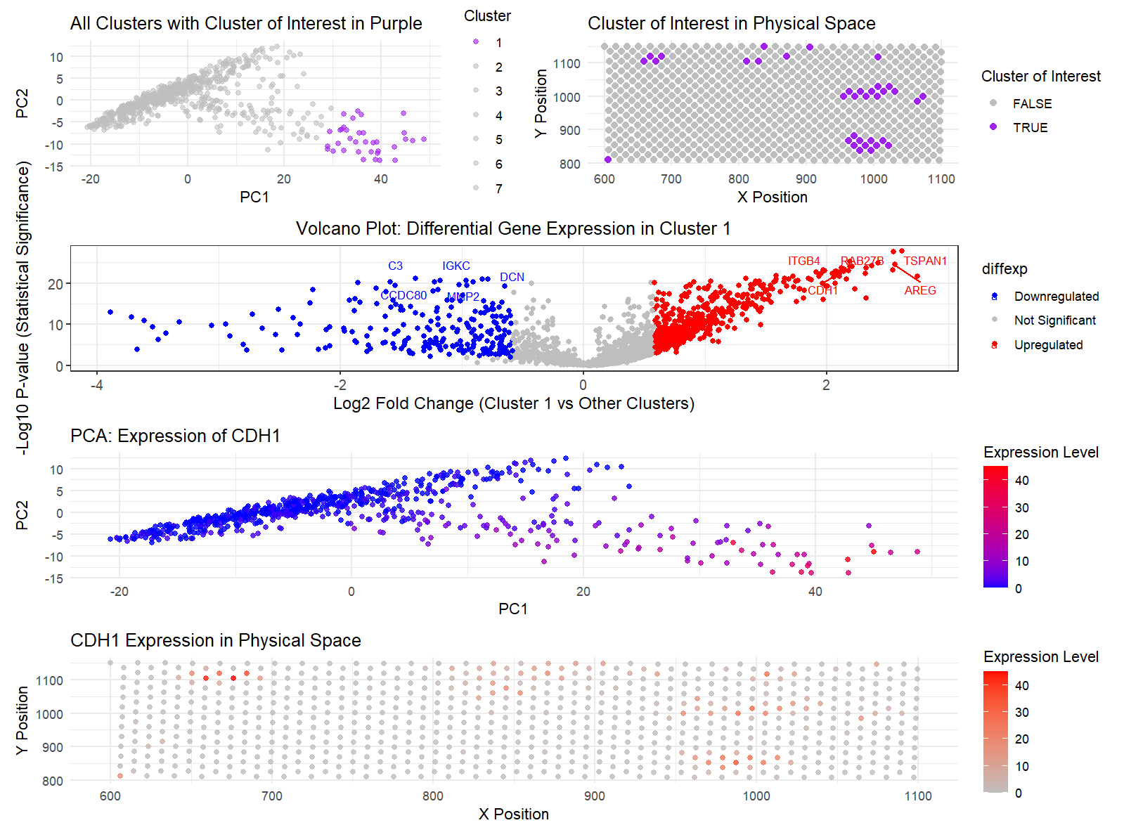
I believe I identified the same cell type, ‘CDH1,’ in the eevee dataset as I had identified in the pikachu dataset. By detecting the specific cluster in which CDH1 was present, I determined it localized to cluster 1. I then examined the spatial distribution of CDH1 expression within the cell and confirmed its upregulation compared to other cells in the diagram. To further validate this, I used PCA to determine the cluster with the highest CDH1 expression and pinpoint the cellular regions where the expression was most prominent. These analyses supported my earlier findings, confirming that CDH1 was present in the dataset.
One of the adjustments I made during the analysis involved re-evaluating the number of clusters. Initially, the Pikachu dataset, analyzed using the elbow method, yielded 5 clusters. However, in this dataset, 7 clusters proved to be more appropriate. I believe the additional clusters were necessary due to the increased complexity of the dataset, likely reflecting greater cellular heterogeneity or more distinct subpopulations with subtle variations in gene expression that were not captured by fewer clusters. Another change I had to implement was modifying plot 3. The original version of the plot did not effectively highlight the upregulation or downregulation of all genes or provide clear identification of which specific genes were upregulated or downregulated. In the updated volcano plot, I ensured that the distribution of gene expression across all genes was clearly visible, with genes of interest—such as CDH1—marked directly on the plot. This adjustment was particularly crucial for comprehending where and if CDH1 was significantly upregulated compared to other genes, as it allowed me to easily pinpoint its position within the distribution and assess its relative expression levels.
Code (paste your code in between the ``` symbols)
1
2
3
4
5
6
7
8
9
10
11
12
13
14
15
16
17
18
19
20
21
22
23
24
25
26
27
28
29
30
31
32
33
34
35
36
37
38
39
40
41
42
43
44
45
46
47
48
49
50
51
52
53
54
55
56
57
58
59
60
61
62
63
64
65
66
67
68
69
70
71
72
73
74
75
76
77
78
79
80
81
82
83
84
85
86
87
88
89
90
91
92
93
94
95
96
97
98
99
100
101
102
103
104
105
106
107
108
109
110
111
112
113
114
115
116
117
118
119
120
121
122
123
124
125
126
127
128
129
130
131
132
133
134
135
136
137
138
139
140
141
142
143
144
145
146
147
148
149
150
151
152
153
154
155
156
157
158
159
160
161
162
163
164
# Packages
library(ggplot2)
library(patchwork)
library(cluster)
library(Rtsne)
#install.packages("ggrepel")
library(dplyr)
library(ggrepel)


# Load data
file <- '/Users/ishit/GenomicVis/genomic-data-visualization-2025/data/eevee.csv.gz'
data <- read.csv(file)
data[1:5, 1:10]
pos <- data[, 3:4]
rownames(pos) <- data$cell_id
gexp <- data[, 7:ncol(data)]
rownames(gexp) <- data$barcode
head(gexp)
head(pos)

#trying different k-means:
# ks = c(5,6,7,8,9,10)
# #around ks = 7 is the elbow
# totw <- sapply(ks, function(k) {
#   print(k)
#   com <- kmeans(gexp, centers=k)
#   return(com$tot.withinss)
# })
# plot(ks, totw)

#normalizing
set.seed(42)
com <- kmeans(loggexp, centers=7)
loggexp <- log10(gexp+1)
com <- kmeans(loggexp, centers=7)
clusters <- com$cluster
clusters <- as.factor(clusters)
names(clusters) <- rownames(gexp)
head(clusters)

pcs <- prcomp(loggexp)

#All Clusters
df <- data.frame(pcs$x, clusters)
ggplot(df, aes(x=PC1, y=PC2, col=clusters)) + geom_point()

gene_cluster_means <- aggregate(loggexp, by = list(cluster = clusters), FUN = mean)

# getting the cluster CDH1 is in
gene_of_interest <- "CDH1"
if (gene_of_interest %in% rownames(gene_cluster_means_t)) {
  assigned_cluster <- names(which.max(gene_cluster_means_t[gene_of_interest, ]))
  print(paste("Gene", gene_of_interest, "is most expressed in", assigned_cluster))
} else {
  print("Gene not found in the dataset!")
}

# Panel 1: Cluster of Interest in PCA (PC1 vs PC2)
selected_cluster <- "1"

cluster_colors <- setNames(rep("grey", length(unique(clusters))), unique(clusters))
cluster_colors[selected_cluster] <- "purple"

panel1 <- ggplot(df, aes(x = PC1, y = PC2, color = clusters)) +
  geom_point(alpha = 0.6) +
  scale_color_manual(values = cluster_colors) +
  theme_minimal() +
  labs(title = "All Clusters with Cluster of Interest in Purple", color = "Cluster")

panel1

# Panel 2: Cluster 1 in Physical Space
pos_df <- data.frame(pos, clusters)
panel2 <- ggplot(pos_df, aes(x=aligned_x, y=aligned_y, col=clusters == selected_cluster)) +
  geom_point(size=2) +
  scale_color_manual(values=c("grey", "purple"), name="Cluster of Interest") +
  labs(title="Cluster of Interest in Physical Space", x="X Position", y="Y Position") +
  theme_minimal()

panel2

#Panel 3: Genes in my cluster of interest
gexpfilter <- gexp[, colSums(gexp) > 1000]
gexpnorm <- log10(gexpfilter / rowSums(gexpfilter) * mean(rowSums(gexpfilter)) + 1)

# Perform the Wilcoxon test and calculate log fold change
pv <- sapply(colnames(gexpnorm), function(i) {
  wilcox.test(gexpnorm[clusters == "1", i], gexpnorm[clusters != "1", i])$p.value
})

logfc <- sapply(colnames(gexpnorm), function(i) {
  log2(mean(gexpnorm[clusters == "1", i]) / mean(gexpnorm[clusters != "1", i]))
})

df_diffexp <- data.frame(gene = colnames(gexpnorm), logfc, logpv = -log10(pv))
df_diffexp$diffexp <- "Not Significant"
df_diffexp[df_diffexp$logpv > 2 & df_diffexp$logfc > 0.58, "diffexp"]
df_diffexp[df_diffexp$logpv > 2 & df_diffexp$logfc < -0.58, "diffexp"]
df_diffexp$diffexp <- as.factor(df_diffexp$diffexp)

upregulated_genes <- df_diffexp %>%
  filter(diffexp == "Upregulated") %>%
  arrange(desc(logpv)) %>%
  head(5)

downregulated_genes <- df_diffexp %>%
  filter(diffexp == "Downregulated") %>%
  arrange(desc(logpv)) %>%
  head(5)

#include CDH1 in the labeled genes
labeled_genes <- bind_rows(upregulated_genes, downregulated_genes) %>%
  bind_rows(df_diffexp %>% filter(gene == "CDH1"))

# volcano plot with labels
p3 <- ggplot(df_diffexp, aes(x = logfc, y = logpv, color = diffexp)) +
  geom_point() +
  geom_text_repel(data = labeled_genes, aes(label = gene), size = 3, box.padding = 0.5) +
  scale_color_manual(values = c("blue", "grey", "red")) +
  ggtitle("Volcano Plot: Differential Gene Expression in Cluster 1") +
  xlab("Log2 Fold Change (Cluster 1 vs Other Clusters)") +
  ylab("-Log10 P-value (Statistical Significance)") +
  theme_bw() +
  theme(plot.title = element_text(hjust = 0.5),
        axis.title = element_text(size = 12),
        axis.text = element_text(size = 10))

# Display the plot
p3


#Panel 4: Picking a gene in the cluster + visualizing in PC1
gene_names <- colnames(gexp)
gene_names
selected_gene <- "CDH1"
df$gene_expression <- gexp[, selected_gene]

df$gene_expression <- gexp[, selected_gene]

panel4 <- ggplot(df, aes(x = PC1, y = PC2, color = gene_expression)) +
  geom_point(size = 1.5, alpha = 0.8) +
  scale_color_gradient(low = "blue", high = "red") +
  labs(title = paste("PCA: Expression of", selected_gene),
       color = "Expression Level") +
  theme_minimal()

panel4

# Panel 5: Gene CDH1 in the physical space
pos_df$CDH1_expression <- data$CDH1
panel5 <- ggplot(pos_df, aes(x = aligned_x, y = aligned_y, col = CDH1_expression)) +
  geom_point(size = 1.5, alpha = 0.8) +
  scale_color_gradient(low = "grey", high = "red") +
  labs(title = "CDH1 Expression in Physical Space",
       color = "Expression Level", x = "X Position", y = "Y Position") +
  theme_minimal()

panel5

# Display all panels
(panel1 + panel2) / (p3) /  (panel4) / panel5