Validating Sequencing-based 10x Visium Identification of T Cell Population with Imaging-Based Spatial Transcriptomics

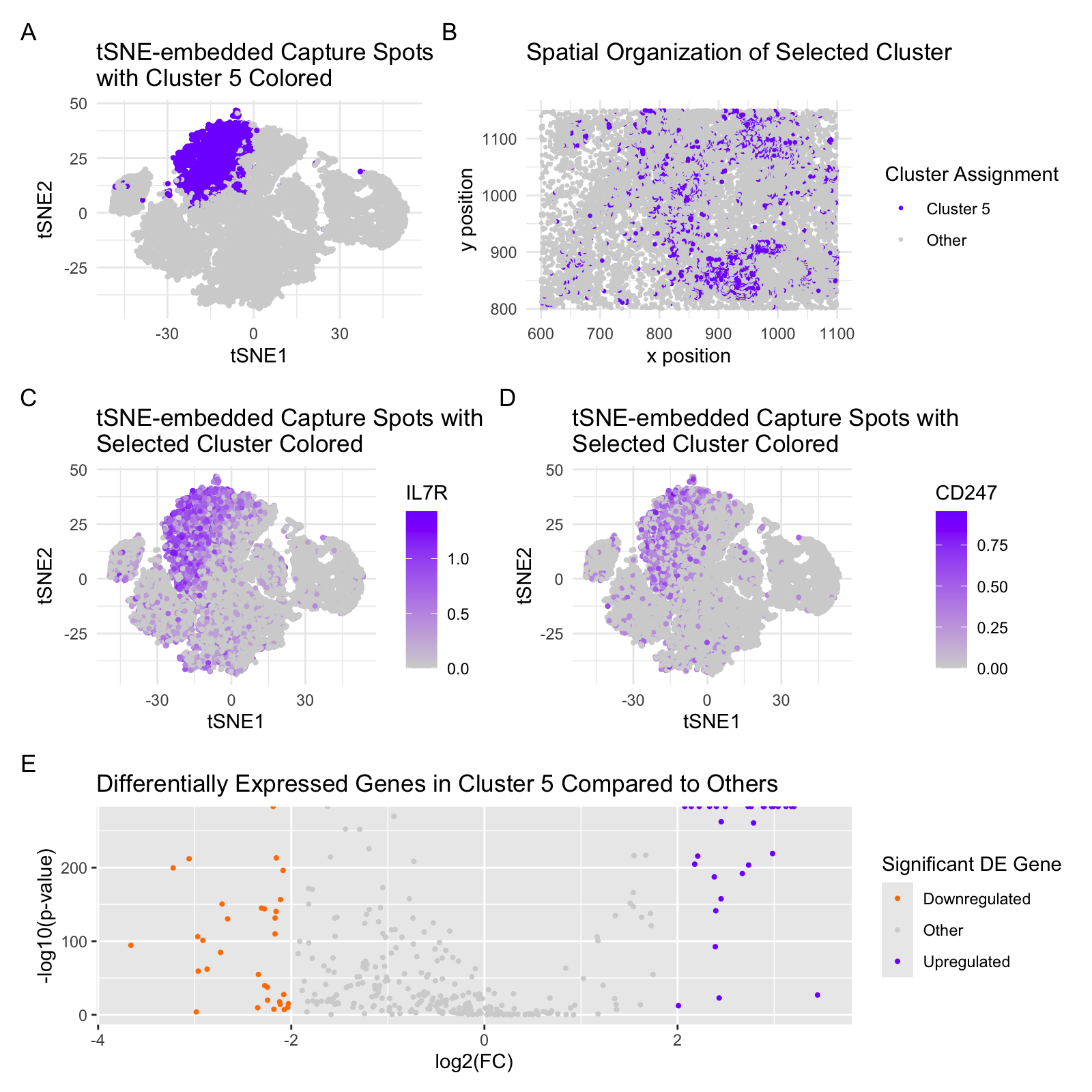
From last week’s results and selected cluster, I identified the genes LTB, CD247, and IL7R , all of which suggest a T cell population (or similar immune cell population comprising B cells). In working with the imaging-based dataset, I applied a similar clustering approach and used selected overexpressed markers to identify a similar cell type cluster. Though LTB was the most strongly correlated hit in the sequencing-based dataset, sparse detection of LTB in the imaging-based set made this an unconvincing marker gene for the selected cell type. I therefore opted to visualize IL7R and CD247, both of which were represented prominently in both the imaging and sequencing-based datasets and suggested a distinct niche in the tSNE-embedded gex space for the imaging-based dataset. Based on this identified location, I tuned the clustering parameters to best fit the intended cell type expression patterns for IL7R and CD247. I thus identified the illustrated cluster 5 as the comparable T cell population. I accordingly adjusted the code to accomodate the reduced gene set and data clustering in the imaging-based dataset. IL7R and CD247 are potent T cell markers. I also opted not to reduce the dataset to the top gene hits, in contrast to the sequencing-based dataset, and saw a significant improvement in clarity of embedding when using tSNE over PCA versus the same two methods used in the sequencing-based set.
5. Code (paste your code in between the ``` symbols)
1
2
3
4
5
6
7
8
9
10
11
12
13
14
15
16
17
18
19
20
21
22
23
24
25
26
27
28
29
30
31
32
33
34
35
36
37
38
39
40
41
42
43
44
45
46
47
48
49
50
51
52
53
54
55
56
57
58
59
60
61
62
63
64
65
66
67
68
69
70
71
72
73
74
75
76
77
78
79
80
81
82
83
84
85
86
87
88
89
90
91
92
93
94
95
96
97
98
99
100
101
102
103
104
105
106
107
108
109
110
111
112
113
114
115
116
117
118
119
120
121
122
123
124
125
126
127
128
129
130
131
132
133
134
135
136
137
138
139
140
141
142
143
144
145
146
147
148
149
150
151
152
153
154
155
156
157
158
159
160
161
162
163
164
165
166
167
168
169
170


## SV Kammula | HW4
## HW4 GDV
## SV Kammula

data <- read.csv('pikachu.csv.gz')

library(ggplot2)
library(patchwork)
library(Rtsne)
library(ggrepel)

pos <- data[, 5:6]
rownames(pos) <- data$X
gexp <- data[, 7:ncol(data)]

norm <- gexp/rowSums(gexp) * 10000
rowSums(norm)

loggexp <- log10(gexp + 1)
com <- kmeans(loggexp, centers = 7)
clusters <- com$cluster
clusters <- as.factor(clusters)
names(clusters) <- rownames (gexp)
head(clusters)

pcs <- prcomp(loggexp)
df <- data.frame(pcs$x, clusters, gene = gexp[, 'CD4'])
ggplot(df, aes(x=PC1, y=PC2, col=clusters)) + geom_point()


ggplot(df, aes(x=PC1, y=PC2, col=gene)) + geom_point()

emb <- Rtsne::Rtsne(pcs$x[,1:10])$Y
head(emb)

pos$clusters <- clusters
ggplot(df, aes(x = emb[,1], y = emb[,2], col=clusters)) + geom_point()

df <- data.frame(emb, clusters, gene = loggexp[, 'IL7R'])
df$clusters_colored <- ifelse(df$clusters == 5, "Cluster 5", "Other")
pos$clusters_colored <- ifelse(pos$clusters == 5, "Cluster 5", "Other")


g1 <- ggplot(df, aes(x = emb[,1], y = emb[,2], col = clusters_colored)) +
  geom_point(size = 0.75) +
  scale_color_manual(values = c("Cluster 5" = "#8000FF", "Other" = "lightgray")) +
  labs(color = "Cluster Assignment") +
  theme_minimal() +
  ggtitle('tSNE-embedded Capture Spots \nwith Cluster 5 Colored') +
  xlab("tSNE1") +
  ylab("tSNE2") +
  theme(legend.position = "none")

g2 <- ggplot(pos, aes(x = aligned_x, y = aligned_y, col = clusters_colored)) +
  geom_point(size = 0.5) +
  scale_color_manual(values = c("Cluster 5" = "#8000FF", "Other" = "lightgray")) +
  labs(color = "Cluster Assignment") +
  ggtitle('Spatial Organization of Selected Cluster') +
  theme_minimal() +
  xlab("x position") +
  ylab("y position")


g3 <- ggplot(df, aes(x = emb[,1], y = emb[,2], col = gene)) +
  geom_point(size = 0.75) +
  scale_color_gradient(high = "#8000FF", low = "lightgray") +
  labs(color = "IL7R") +
  theme_minimal() +
  ggtitle('tSNE-embedded Capture Spots with \nSelected Cluster Colored') +
  xlab("tSNE1") +
  ylab("tSNE2")

df <- data.frame(emb, clusters, gene = loggexp[, 'LTB'])
g4 <- ggplot(df, aes(x = emb[,1], y = emb[,2], col = gene)) +
  geom_point(size = 0.75) +
  scale_color_gradient(high = "#8000FF", low = "lightgray") +
  labs(color = "LTB") +
  theme_minimal() +
  ggtitle('tSNE-embedded Capture Spots with \nSelected Cluster Colored') +
  xlab("tSNE1") +
  ylab("tSNE2")


df <- data.frame(emb, clusters, gene = loggexp[, 'CXCR4'])
g5 <- ggplot(df, aes(x = emb[,1], y = emb[,2], col = gene)) +
  geom_point(size = 0.75) +
  scale_color_gradient(high = "#8000FF", low = "lightgray") +
  labs(color = "CXCR4") +
  theme_minimal() +
  ggtitle('tSNE-embedded Capture Spots with \nSelected Cluster Colored') +
  xlab("tSNE1") +
  ylab("tSNE2")

df <- data.frame(emb, clusters, gene = loggexp[, 'CD247'])
g6 <- ggplot(df, aes(x = emb[,1], y = emb[,2], col = gene)) +
  geom_point(size = 0.75) +
  scale_color_gradient(high = "#8000FF", low = "lightgray") +
  labs(color = "CD247") +
  theme_minimal() +
  ggtitle('tSNE-embedded Capture Spots with \nSelected Cluster Colored') +
  xlab("tSNE1") +
  ylab("tSNE2")

#df <- data.frame(emb, clusters, gene = loggexp[, 'PTPN22'])
#g5 <- ggplot(df, aes(x=emb[,1], y=emb[,2], col=gene)) + geom_point(size = .5)


## differential gene expression analysis

interest <- 5
cellsOfInterest <- names(clusters)[clusters == interest]
otherCells <- names(clusters)[clusters != interest]
i <- 'CD4' #find on expressed in cluster of interest
genetest <- norm[,i]
names(genetest) <- rownames(norm)
genetest[cellsOfInterest]
genetest[otherCells]
t.test(genetest[cellsOfInterest], genetest[otherCells], )


# differential gene expression
pvalues <- sapply(colnames(norm), function(i) {
  wilcox.test(gexp[clusters == 5, i], gexp[clusters != 5, i])$p.val
})

# get log fold change
logfc <- sapply(colnames(gexp), function(i) {
  log2(mean(norm[clusters == 5, i])/mean(norm[clusters != 5, i]))
})

valid_indices <- !is.na(pvalues)
filtered_pvalues = pvalues[valid_indices]
filtered_logfc = logfc[valid_indices]


# volcano plot
df_volc = data.frame(pvalues = -log10(filtered_pvalues), log_fc = filtered_logfc)
df_volc$genes <- rownames(df_volc)


#df_volc_cleaned <- df_volc[!is.nan(df_volc$p_values) & !is.nan(df_volc$logFC), ]
upper_logfc <- 2
lower_logfc <- -2

df_volc$color <- ifelse(df_volc$log_fc > upper_logfc, "Upregulated",
                        ifelse(df_volc$log_fc < lower_logfc, "Downregulated", "Other"))


g7 <- ggplot(df_volc, aes(x = log_fc, y = pvalues, color = color)) +
  geom_point(size= 0.75) +
  ggtitle("Differentially Expressed Genes in Cluster 5 Compared to Others") +
  scale_color_manual(values = c("Upregulated" = "#8000FF",
                                "Downregulated" = "#FF8000",
                                "Other" = "lightgray")) +
  labs(color = "Significant DE Gene") +
#scale_color_manual(values = c("Cluster 3" = "#8000FF", "Other" = "lightgray")) +
  xlab("log2(FC)") +
  ylab("-log10(p-value)")

(g1 + g2) / (g3 + g6) / g7 + plot_annotation(tag_levels = 'A')


###