HW4: Exploring Cell Type with Differentially upregulated CD4

1. Figure Description.
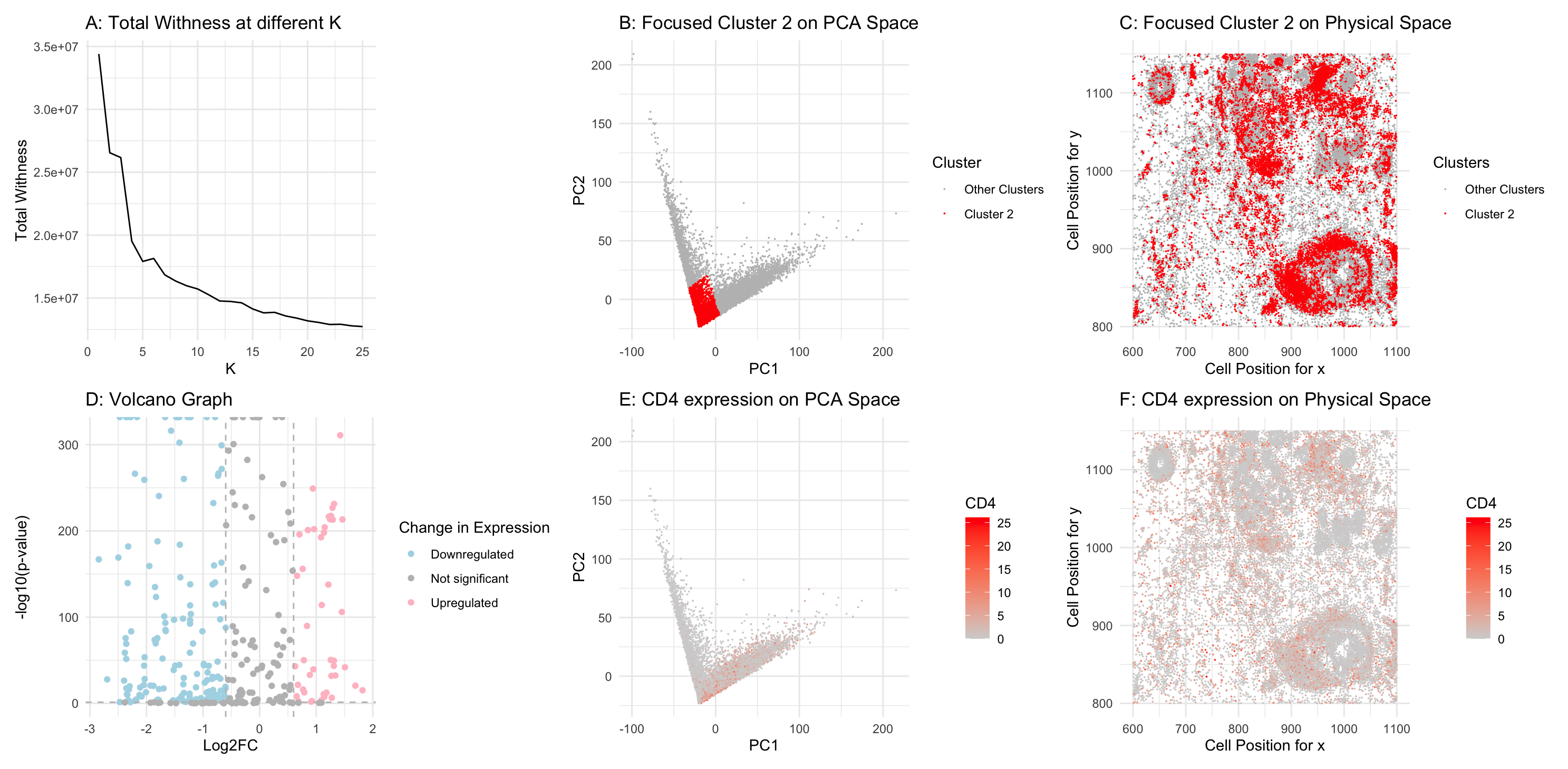
Figure A: Total within-cluster sum of squares using different value of k. Figure B: Cluster 2 is highlighted in red in PCA space, while the remaining three clusters are shown in grey. The axes represent PC1 and PC2. Figure C: Cluster 2 is highlighted in red to show its distribution in physical space, with the remaining six clusters in grey. The axes represent x and y spot positions. Figure D: A volcano plot comparing gene expression in Cluster 2 versus the other clusters. The y-axis represents p-values in -log10 scale, while the x-axis represents log2 fold changes between Cluster 2 and the rest of the clusters. Figure E: CD4 gene expression is visualized in PCA space, highlighted in a gradient red. Figure F: CD4 gene expression is visualized in physical space, highlighted in a gradient red.
2. Cluster interpretation.
My analysis shows that Cluster 2 cells exhibit differentially upregulated CD4, a key marker for helper T cells. This conclusion is supported by both the differential gene expression analysis and the visualizations in Figures B and E, where Cluster 2 displays the highest CD4 expression level in PCA space. Additionally, in Figures C and F, cells in Cluster 2 show high CD4 expression in the same physical space.
Therefore, Cluster 2 must represent helper T cells, confirming the same cell type I identified in my previous assignment.
3. Changes I made for pikachu dataset.
I used volume normalization with cell size instead of count normalization because this is an imaging-based spatial omics dataset. In contrast, the Eevee dataset is spot-based, so count normalization was more appropriate in the previous method.
Previously, I generated the total within-cluster sum of squares vs. k graph for the Eevee dataset and used the elbow method to determine that k = 7 was the optimal cluster number. Applying the same method to the Pikachu dataset, I found that k = 4 is more appropriate. I believe this is because the number of genes in this dataset is smaller, leading to a lower total within-cluster sum of squares at a smaller k value.
Additionally, this dataset does not include the gene CD52, which I analyzed in a previous assignment, likely due to the limitations of the imaging-based method. Instead, I focused on CD4, a marker I also previously examined, to confirm that cluster 2 corresponds to the same helper T cells identified in my earlier work.
Lastly, I adjusted the point size to 0.01 because the number of cells in this dataset is too large to visualize all at the default size. In contrast, the previous dataset had a small number of spots, so adjusting point size was unnecessary.
4. Citation.
https://clinicalinfo.hiv.gov/en/glossary/cd4-t-lymphocyte#:~:text=A%20type%20of%20lymphocyte.,cells)%2C%20to%20fight%20infection.
5. Code
1
2
3
4
5
6
7
8
9
10
11
12
13
14
15
16
17
18
19
20
21
22
23
24
25
26
27
28
29
30
31
32
33
34
35
36
37
38
39
40
41
42
43
44
45
46
47
48
49
50
51
52
53
54
55
56
57
58
59
60
61
62
63
64
65
66
67
68
69
70
71
72
73
74
75
76
77
78
79
80
81
82
83
84
85
86
87
88
89
90
91
92
93
94
95
96
97
98
99
100
101
102
103
104
105
106
107
108
109
110
111
112
113
114
115
116
117
118
119
120
121
122
library(ggplot2)
library(patchwork)

file <- "~/Downloads/pikachu.csv.gz"
data <- read.csv(file)
data[1:5,1:10]

pos <- data[, 5:6]
rownames(pos) <- data$cell_id
gexp <- data[, 7:ncol(data)]
rownames(gexp) <- data$barcode

gexp[1:5, 1:10]
dim(gexp)

# normalization
norm <- gexp/log10(data$cell_area+1) * 3
norm[1:5,1:5]
dim(norm)

## kmeans
ks = 1:25
totw <- sapply(ks, function(k) {
  print(k)
  com <- kmeans(norm, centers=k)
  return(com$tot.withinss)
})


df <- data.frame(ks, totw)
g6 <- ggplot(df, aes(x = ks, y = totw)) +
  geom_line() +
  labs(title = "A: Total Withness at different K",
       x = "K",
       y = "Total Withness"
       ) +
  theme_minimal()


# pick k = 7
com <- kmeans(norm, centers=4)
clusters <- com$cluster
clusters <- as.factor(clusters)
names(clusters) <- rownames(norm)
head(clusters)

# PCA
pcs <- prcomp(norm)
df <- data.frame(pcs$x,clusters)
ggplot(df, aes(x=PC1, y=PC2, col= clusters)) + geom_point()

g1 <- ggplot(df, aes(x=PC1, y=PC2, col= factor(clusters==4, labels = c("Other Clusters","Cluster 2")))) +
  geom_point(size = 0.01) +
  scale_color_manual(values = c("Cluster 2" = "red", "Other Clusters" = "grey"))+
  labs(title = "B: Focused Cluster 2 on PCA Space", col = "Cluster") +
  theme_minimal()


df <- data.frame(pos,norm,clusters)
g2<- ggplot(df, aes(x = aligned_x, y = aligned_y, col = factor(clusters==4, labels = c("Other Clusters","Cluster 2")))) +
  geom_point(size = 0.01) +
  scale_color_manual(values = c("Cluster 2" = "red", "Other Clusters" = "grey"))+
  labs(title = "C: Focused Cluster 2 on Physical Space", col = "Clusters",
       x = "Cell Position for x",
       y = "Cell Position for y") +
  theme_minimal()

# differential expression
cellsOfInterest <- names(clusters)[clusters == 4]
otherCells <- names(clusters)[clusters != 4]

results <- sapply(1:ncol(norm), function(i) {
  genetest <- norm[,i]
  names(genetest) <- rownames(norm)
  out <- t.test(genetest[cellsOfInterest], genetest[otherCells], alternative = 'two.side')
  out$p.value
})

names(results) <- colnames(norm)
results <- sort(results, decreasing = FALSE)
length(results)


Cluster1Cell <- norm[cellsOfInterest,]
SumCluster1Cell <- colSums(Cluster1Cell)/length(cellsOfInterest)

OtherClustersCell <- norm[otherCells,]
SumOtherClustersCell <- colSums(OtherClustersCell)/length(otherCells)

log_results <- -log10(results)
log_2FC <- log2(SumCluster1Cell/SumOtherClustersCell)

df <- data.frame(log_results, log_2FC)
df$diffexpressed <- "NO"
df$diffexpressed[df$log_2FC > 0.6 & df$log_results > -log10(0.05)] <- "UP"
df$diffexpressed[df$log_2FC < -0.6 & df$log_results > -log10(0.05)] <- "DOWN"

g3 <-   ggplot(df, aes(y=(log_results), x = log_2FC, col = diffexpressed)) + geom_point() +
  geom_vline(xintercept = c(-0.6, 0.6), col = "gray", linetype = 'dashed') +
  geom_hline(yintercept = -log10(0.05), col = "gray", linetype = 'dashed') +
  labs(title = "D: Volcano Graph",
       y = "-log10(p-value)",
       x = "Log2FC", col = "Change in Expression") +
  scale_color_manual(values = c("lightblue", "grey", "pink"),
                     labels = c("Downregulated", "Not significant", "Upregulated"))+
  theme_minimal()

# one gene in PCA
df <- data.frame(pcs$x, clusters, gene = norm[, 'CD4'])
g4 <- ggplot(df, aes(x=PC1, y=PC2, col=gene)) + labs(title = "E: CD4 expression on PCA Space", col = "CD4") +
  scale_color_gradient(low = 'lightgrey', high = 'red') + geom_point(size = 0.01) + theme_minimal()

# one gene in physical space
df <- data.frame(pos, gene = norm[,"CD4"])
g5 <- ggplot(df, aes(x = aligned_x, y = aligned_y, col = gene)) +
  labs(title = "F: CD4 expression on Physical Space ",
       x = "Cell Position for x",
       y = "Cell Position for y",
       col = "CD4") + scale_color_gradient(low = 'lightgrey', high = 'red') +
  geom_point(size = 0.01) + theme_minimal()

g6 + g1 + g2 + g3 + g4 + g5