HW5

Hi I'm Siddhi

Description:

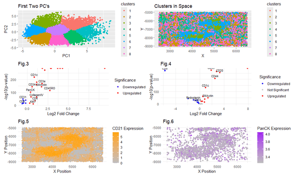
For this assignment, I first started out by following similar steps to my previous homeworks - normalizing the data, performing kmeans clustering by using the optimal k value, visualizing my results in pca space, and performing differential expression analysis (via the wilcox test) for upregulation and downregulation. I visualized the cluster data in spatial position as well as sanity checks. However, I noticed when visualizing in PCA space, that the kmeans clustering seemed quite scattered, and it seemed a little scattered when plotted in spatial locations as well. Due to this, I reduced the dimensionality of the data by applying PCA first, and then I performed kmeans clustering on the reduced data. I followed the other steps in the same order as previous after this step. I found through this method that the visualizations of clustering in space were more distinct. Thus I decided that this methodology, reducing dimensionality and then performing clustering, would be more suitable for the needs of this assignment, especially given how little we know about the dataset.
Figures 1 and 2 show the clustering in PC space and xy space respectively. Figures 3 and 4 display differential expression levels in the logarithmic scale for clusters 6 and 3 respectively. Figure 5 shows the upregulated CD21 expression in cluster 6, which very distinctly matches the region I want to capture. This visually indicates a strong relation between CD21 and my cell cluster of interest. Figure 6 shows PanCK upregulation expression in areas that also have downregulated CD31. Through iterations, I discovered that plotting both of these was necessary to get a visual representation specific to my cluster of interest. This shows an interesting characteristic of the data, specifically that in cluster 3, BOTH the CD31 downregulation and PanCK upregulation are needed to accurately characterize the cell. I am confident in my results, as I followed a consistent process and performed careful checks along the way. I performed dimensionality reduction on the data, then kmeans clustering, making sure to plot the total withinness for different k values before settling on the optimal “elbow” value fo k=8. Then I performed the wilcox tests for both upregulation and downregulation in my clusters of interest. Identifying the most statistically significant upregulation and downregulation allow me to make a stronger correlation to cell type, rather than just focusing on only up or down regulation. I also plotted my upregulation and downregulation spatially as a “sanity check” and made sure they match my original spatial clustering. I decided to investigate clusters 6 and 3. I picked these from my spatial visualization of clustering (Fig2.), as upon visual inspection they appear to be the most distinctly shaped structures. In cluster 6, I found the CD21 and Podoplanin to be among the most upregulated, and the CD31 and Lyve1 to be among the most downregulated. Literature suggests that upregulation of Podoplanin highly corresponds to Follicular Dendritic cells and so does CD21 upregulation, and downregulation of CD31 corresponds to T Lymphocytes, and downregulation of Lyve1 corresponds to lymphatic cells. Thus I suspect this cluster to be lymph cells, as FDC’s are found in B cell follicles of secondary lymphoid organs. In cluster 3, I found the PanCK and SMActin to be among the most upregulated, and the Ki67 and CD45RO to be among the most downregulated. Literature suggests that upregulation of PanCK and SMActin corresponds to endothelial cells, and downregulation of Ki67 can be associated with quiescent endothelial cells. CD45RO downregulation highly suggests this cell is not a T cell or an immune cell. Thus I suspect cluster 3 to be endothelial cells. Due to my findings indicative of T Lymphocytes and endothelial cell types, I would say that this tissue structure most represents white pulp, likely found in the spleen.

Sources:

https://pmc.ncbi.nlm.nih.gov/articles/PMC2196095/ https://pubmed.ncbi.nlm.nih.gov/18838918/ https://pubmed.ncbi.nlm.nih.gov/1544907/#:~:text=activated%20T%20lymphocytes-,The%20cell%20adhesion%20molecule%20CD31%20is%20phosphorylated%20after%20cell%20activation,(8):5243%2D9. https://www.jbc.org/article/S0021-9258(20)71702-3/pdf#:~:text=3B).,either%20transcription%20or%20mRNA%20turnover. https://journals.aai.org/jimmunol/article/160/3/1078/31037/Follicular-Dendritic-Cell-FDC-Precursors-in https://www.nature.com/articles/s41586-021-03570-8 https://www.ahajournals.org/doi/10.1161/CIRCULATIONAHA.121.055417#:~:text=Endothelial%20to%20mesenchymal%20transition%20(EndoMT)%20is%20a%20process%20of%20cell,are%20descendants%20of%20endocardial%20ECs. https://www.spandidos-publications.com/10.3892/ol.2015.3286 https://www.frontiersin.org/journals/immunology/articles/10.3389/fimmu.2012.00201/full

Code:

library(ggplot2)
library(patchwork)
file <- 'C:\\Hopkins School Stuff\\GenomicDataVis\\data\\codex_spleen_3.csv.gz'
data <- read.csv(file)
data[1:5,1:10]
pos <- data[, 2:3]
rownames(pos) <- data$cell_id
head(pos)
area <-data[,4]
gexp <- data[, 5:ncol(data)]
rownames(gexp) <- data$barcode
head(gexp)
head(pos)

norm <-log10(gexp/rowSums(gexp) * 1e6 +1)
norm[1:5,1:5]


ks = c(2,3,4,5,6,7,8,9,10,11, 12, 13, 14, 15, 16)
totw <-sapply(ks,function(k){
  print(k)
  com <-kmeans(norm,centers=k)
  return(com$tot.withinss)
})
plot(ks,totw)
ggplot(pos, aes(x=x, y=y)) + geom_point()
##looks like elbow is at k=8, pick k=8
com <-kmeans(norm, centers=8)
clusters <- com$cluster
clusters <- as.factor(clusters)
names(clusters) <-rownames(gexp)
head(clusters)

pcs <-prcomp(norm)
df <- data.frame(pcs$x, clusters)
head(pcs)
pc_plot<-ggplot(df, aes(x=PC1, y=PC2, col=clusters)) + geom_point()+ labs(title = "PC's")
pc_plot
## Now Try doing PCA first, then clustering on the first two PC's

pcs <- prcomp(norm)
plot(pcs$sdev)
elbow <- sapply(2:20, function(k) {
  out <- kmeans(pcs$x[,1:2], centers=k)
  out$tot.withinss
})
plot(2:20, elbow)

clusters <- as.factor(kmeans(pcs$x[,1:2], centers=8)$cluster)
df <- data.frame(pcs$x[,1:2], clusters)
PC_PLOT<-ggplot(df, aes(x = PC1, y=PC2, col=clusters)) + geom_point()
df <- data.frame(pos, clusters)
SPAT_PLOT<-ggplot(df, aes(x = x, y=y, col=clusters)) + geom_point()
PC_PLOT
SPAT_PLOT

names(clusters) <- rownames(norm)  
ct1 <- names(clusters)[which(clusters == interest)]
ctother <- names(clusters)[which(clusters != interest)]
results <- sapply(colnames(norm), function(i) {
  wilcox.test(norm[ct1, i], norm[ctother, i], alternative = 'greater')$p.value ##upregulated
})
names(results) <- colnames(norm)
post_pcaClust_results<-sort(results[results < 0.05/ncol(norm)])

names(results) <- colnames(norm)
sort(results[results < 0.05/ncol(colnames)])


## Now Try doing PCA first, then clustering on the first two PC's

pcs <- prcomp(norm)
plot(pcs$sdev)
elbow <- sapply(2:20, function(k) {
  out <- kmeans(pcs$x[,1:2], centers=k)
  out$tot.withinss
})
plot(2:20, elbow)

clusters <- as.factor(kmeans(pcs$x[,1:2], centers=8)$cluster)
df <- data.frame(pcs$x[,1:2], clusters)
PC_PLOT<-ggplot(df, aes(x = PC1, y=PC2, col=clusters)) + geom_point()
df <- data.frame(pos, clusters)
SPAT_PLOT<-ggplot(df, aes(x = x, y=y, col=clusters)) + geom_point()
PC_PLOT
SPAT_PLOT

names(clusters) <- rownames(norm)  
ct1 <- names(clusters)[which(clusters == interest)]
ctother <- names(clusters)[which(clusters != interest)]
results <- sapply(colnames(norm), function(i) {
  wilcox.test(norm[ct1, i], norm[ctother, i], alternative = 'greater')$p.value ##upregulated
})
names(results) <- colnames(norm)
post_pcaClust_results<-sort(results[results < 0.05/ncol(norm)])

names(results) <- colnames(norm)
sort(results[results < 0.05/ncol(colnames)])


## for cluster 6
interest<-6
names(clusters) <- rownames(norm)  
ct1 <- names(clusters)[which(clusters == interest)]
ctother <- names(clusters)[which(clusters != interest)]
results <- sapply(colnames(norm), function(i) {
  wilcox.test(norm[ct1, i], norm[ctother, i], alternative = 'greater')$p.value ##upregulated
})
names(results) <- colnames(norm)
clust6_upreg<-sort(results[results < 0.05/ncol(norm)])

results <- sapply(colnames(norm), function(i) {
  wilcox.test(norm[ct1, i], norm[ctother, i], alternative = 'less')$p.value ##downregulated
})
names(results) <- colnames(norm)
clust6_downreg<-sort(results[results < 0.05/ncol(norm)])

clust6_upreg
clust6_downreg


## for cluster 3

interest<-3
names(clusters) <- rownames(norm)  
ct1 <- names(clusters)[which(clusters == interest)]
ctother <- names(clusters)[which(clusters != interest)]
results <- sapply(colnames(norm), function(i) {
  wilcox.test(norm[ct1, i], norm[ctother, i], alternative = 'greater')$p.value ##upregulated
})
names(results) <- colnames(norm)
clust3_upreg<-sort(results[results < 0.05/ncol(norm)])

results <- sapply(colnames(norm), function(i) {
  wilcox.test(norm[ct1, i], norm[ctother, i], alternative = 'less')$p.value ##downregulated
})
names(results) <- colnames(norm)
clust3_downreg<-sort(results[results < 0.05/ncol(norm)])

clust3_upreg
clust3_downreg


library(ggplot2)
##clust 6 volcano plot
interest <- 6
names(clusters) <- rownames(norm)
ct1 <- names(clusters)[which(clusters == interest)]
ctother <- names(clusters)[which(clusters != interest)]
upreg_results_6 <- sapply(colnames(norm), function(i) {
  wilcox.test(norm[ct1, i], norm[ctother, i], alternative = 'greater')$p.value
})
names(upreg_results_6) <- colnames(norm)
clust6_upreg <- sort(upreg_results_6[upreg_results_6 < 0.05 / ncol(norm)])
downreg_results_6 <- sapply(colnames(norm), function(i) {
  wilcox.test(norm[ct1, i], norm[ctother, i], alternative = 'less')$p.value
})
names(downreg_results_6) <- colnames(norm)
clust6_downreg <- sort(downreg_results_6[downreg_results_6 < 0.05 / ncol(norm)])

mean_ct1_6 <- colMeans(norm[ct1, , drop = FALSE])
mean_ctother_6 <- colMeans(norm[ctother, , drop = FALSE])
log2FC_6 <- (mean_ct1_6 - mean_ctother_6) * log2(10)

p_values_6 <- sapply(colnames(norm), function(i) {
  wilcox.test(norm[ct1, i], norm[ctother, i], alternative = 'two.sided')$p.value
})
neg_log10_pval_6 <- -log10(p_values_6)

volcano_data_6 <- data.frame(
  Gene = colnames(norm),
  log2FC = log2FC_6,
  p_value = p_values_6,
  neg_log10_pval = neg_log10_pval_6
)

volcano_data_6$Significance <- "Not Significant"
volcano_data_6$Significance[volcano_data_6$p_value < 0.05 / ncol(norm) & volcano_data_6$log2FC > 0] <- "Upregulated"
volcano_data_6$Significance[volcano_data_6$p_value < 0.05 / ncol(norm) & volcano_data_6$log2FC < 0] <- "Downregulated"

volc_6<-ggplot(volcano_data_6, aes(x = log2FC, y = neg_log10_pval, color = Significance)) +
  geom_point(alpha = 0.8) +
  scale_color_manual(values = c("Upregulated" = "red", "Downregulated" = "blue", "Not Significant" = "gray")) +
  theme_minimal() +
  xlab("Log2 Fold Change") +
  ylab("-log10(p-value)") +
  ggtitle("Fig.3") +
  theme(legend.position = "right") +
  geom_text(aes(label = ifelse(Significance %in% c("Upregulated", "Downregulated"), Gene, "")),
            vjust = -0.5, size = 3, color = "black", check_overlap = TRUE)


##clust 3 volcano plot
interest <- 3
names(clusters) <- rownames(norm)
ct1 <- names(clusters)[which(clusters == interest)]
ctother <- names(clusters)[which(clusters != interest)]

upreg_results_3 <- sapply(colnames(norm), function(i) {
  wilcox.test(norm[ct1, i], norm[ctother, i], alternative = 'greater')$p.value
})
names(upreg_results_3) <- colnames(norm)
clust3_upreg <- sort(upreg_results_3[upreg_results_3 < 0.05 / ncol(norm)])

downreg_results_3 <- sapply(colnames(norm), function(i) {
  wilcox.test(norm[ct1, i], norm[ctother, i], alternative = 'less')$p.value
})
names(downreg_results_3) <- colnames(norm)
clust3_downreg <- sort(downreg_results_3[downreg_results_3 < 0.05 / ncol(norm)])

mean_ct1_3 <- colMeans(norm[ct1, , drop = FALSE])
mean_ctother_3 <- colMeans(norm[ctother, , drop = FALSE])
log2FC_3 <- (mean_ct1_3 - mean_ctother_3) * log2(10)

p_values_3 <- sapply(colnames(norm), function(i) {
  wilcox.test(norm[ct1, i], norm[ctother, i], alternative = 'two.sided')$p.value
})
neg_log10_pval_3 <- -log10(p_values_3)

volcano_data_3 <- data.frame(
  Gene = colnames(norm),
  log2FC = log2FC_3,
  p_value = p_values_3,
  neg_log10_pval = neg_log10_pval_3
)

volcano_data_3$Significance <- "Not Significant"
volcano_data_3$Significance[volcano_data_3$p_value < 0.05 / ncol(norm) & volcano_data_3$log2FC > 0] <- "Upregulated"
volcano_data_3$Significance[volcano_data_3$p_value < 0.05 / ncol(norm) & volcano_data_3$log2FC < 0] <- "Downregulated"

volc_3<-ggplot(volcano_data_3, aes(x = log2FC, y = neg_log10_pval, color = Significance)) +
  geom_point(alpha = 0.8) +
  scale_color_manual(values = c("Upregulated" = "red", "Downregulated" = "blue", "Not Significant" = "gray")) +
  theme_minimal() +
  xlab("Log2 Fold Change") +
  ylab("-log10(p-value)") +
  ggtitle("Fig.4") +
  theme(legend.position = "right") +
  geom_text(aes(label = ifelse(Significance %in% c("Upregulated", "Downregulated"), Gene, "")),
            vjust = -0.5, size = 3, color = "black", check_overlap = TRUE)


##verifying via spatial plotting 

## Cluster 6 - Upregulation

cd21_expr <- norm[, "CD21"]  

df_spatial <- data.frame(pos, clusters, CD21 = cd21_expr, Podoplanin = podoplanin_expr)

# Spatial plot for CD21 expression
clust_6_proof<-ggplot(df_spatial, aes(x = x, y = y, color = CD21)) +
  geom_point() +
  scale_color_gradient(low = "gray", high = "orange") +
  labs(title = "Fig.5", 
       x = "X Position", y = "Y Position", color = "CD21 Expression") +
  theme_minimal() +
  theme(legend.position = "right")


## Cluster 3

panck_expr <- norm[, "PanCK"]  
df_spatial <- data.frame(pos, clusters, PanCK = panck_expr)

# Spatial plot for PanCK expression across all clusters
ggplot(df_spatial, aes(x = x, y = y, color = PanCK)) +
  geom_point() +
  scale_color_gradient(low = "gray", high = "purple") +  # Upregulation color scheme
  labs(title = "Spatial Distribution of PanCK Expression (Up)", 
       x = "X Position", y = "Y Position", color = "PanCK Expression") +
  theme_minimal() +
  theme(legend.position = "right")


cd31_expr <- norm[, "CD31"]  
df_spatial <- data.frame(pos, clusters, CD31 = cd31_expr)

# Spatial plot for CD31 expression across all clusters 
ggplot(df_spatial, aes(x = x, y = y, color = CD31)) +
  geom_point() +
  scale_color_gradient(low = "purple", high = "gray") +  
  labs(title = "Spatial Distribution of CD31 Expression (Down)", 
       x = "X Position", y = "Y Position", color = "CD31 Expression") +
  theme_minimal() +
  theme(legend.position = "right")


# Spatial plot for cells with upregulation of PanCK and downregulation of CD31
panck_expr <- norm[, "PanCK"]
cd31_expr <- norm[, "CD31"]
panck_upregulated <- panck_expr > median(panck_expr)
cd31_downregulated <- cd31_expr < median(cd31_expr)
selected_cells <- panck_upregulated & cd31_downregulated
df_spatial_selected <- data.frame(pos[selected_cells, ], clusters[selected_cells], 
                                  PanCK = panck_expr[selected_cells], CD31 = cd31_expr[selected_cells])

clust3_proof<-ggplot(df_spatial_selected, aes(x = x, y = y, color = PanCK)) +
  geom_point() +
  scale_color_gradient(low = "gray", high = "purple") +  
  labs(title = "Fig.6", 
       x = "X Position", y = "Y Position", color = "PanCK Expression") +
  theme_minimal() +
  theme(legend.position = "right")




library(patchwork)
# Combine plots using patchwork
final_plot <- (PC_PLOT | SPAT_PLOT) / 
  (volc_6 | volc_3) / 
  (clust_6_proof | clust3_proof)

# Display the final combined plot
final_plot

26 Feb 2025

« Uncovering spleen tissue type Identifying cell types in COSEX dataset »