Identifying Unknown Tissue Structure in the Spleen

Create a data visualization and write a description to convince me that your interpretation is correct. Your description should reference papers and content that allowed you to interpret your cell clusters as a particular cell-types. You must provide attribution to external resources referenced. Links are fine; formatted references are not required.
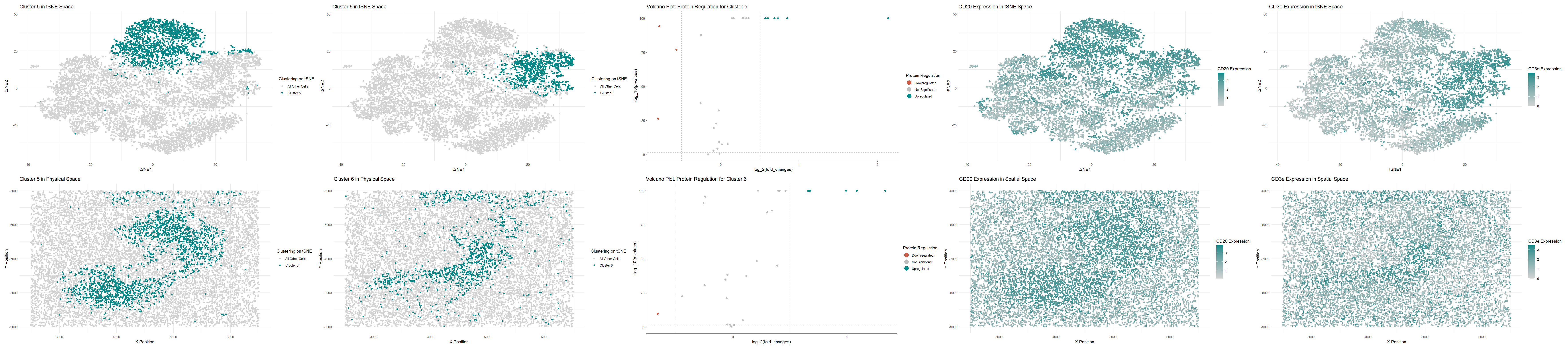
Cluster 5 Upregulated Proteins: CD20, Podoplanin, CD21, CD35, CD44, ECAD, HLA-DR
Cluster 6 Upregulated Proteins: CD3e, CD21, CD4, CD45RO, CD45
CD20 is a protein found in B cells [1]. Podoplanin is expressed in T cells [2] CD21 is also very upregulated in B cells within the spleen [3,9]. CD35 is expressed in B cells and Macrophages within the spleen [4]. CD44 has medium expression in both white pulp and red pulp of the spleen [5]. HLA-DR has medium expression in white pulp of the spleen [6]. According to [7], white pulp consists primarily of B cells and T cells, so analysis of Cluster 5 suggests that we are looking at white pulp.
CD3e is a protein only found in the red pulp of the spleen [8]. CD21 is a protein with high expression only found the white pulp of the spleen [3,9]. CD4 is found in both red and white pulp with medium and low expression, respectively [10]. CD45RO is expressed in T cells [11]. CD45 has very high expression in the both red and white pulp of the spleen, expressed in T cells [12, 13]. Based on our analysis of Cluster 6, we are likely looking at white pulp and some red pulp. Quickly plotting at CD21 expression spatially (not shown on the picture above), we see that it is quite high in the middle structure. CD3e (shown on the picture above), on the other hand, is quite high around all of the tissue besides that middle structure. Therefore, we can make a good conclude that we are likely looking at white pulp surrounded by some red pulp.
So, to answer the question for this homework, since the most relevant tissue structure we are looking at seems to be the blob in the middle, we are looking at (2) White pulp.
Relevant links:
[1] https://www.cancer.gov/publications/dictionaries/cancer-terms/def/cd20
[2] https://pmc.ncbi.nlm.nih.gov/articles/PMC3439854/
[3] https://www.proteinatlas.org/ENSG00000117322-CR2/single+cell/spleen
[4] https://www.proteinatlas.org/ENSG00000203710-CR1/single+cell/spleen
[5] https://www.proteinatlas.org/ENSG00000026508-CD44/tissue/spleen
[6] https://www.proteinatlas.org/ENSG00000204287-HLA-DRA/tissue/spleen
[7] https://www.nature.com/articles/nri1669
[8] https://www.proteinatlas.org/ENSG00000198851-CD3E/tissue/spleen
[9] https://www.proteinatlas.org/ENSG00000117322-CR2/tissue/spleen
[10] https://www.proteinatlas.org/ENSG00000010610-CD4/tissue/spleen
[11] https://pmc.ncbi.nlm.nih.gov/articles/PMC5483817/
[12] https://www.proteinatlas.org/ENSG00000081237-PTPRC/tissue/spleen
[13] https://www.proteinatlas.org/ENSG00000081237-PTPRC/single+cell/spleen
Code
### Ayan Vaishnav
### Genomic Data Visualization 2025
### Homework Assignment 5
### Spatial Proteomics!

## Source for most of the initial code: Ayan's HW4

## Load the libraries
library(ggplot2)
library(patchwork)
library(tidyverse)
library(Rtsne)

set.seed(6)

## Load data
file <- "~/Desktop/genomic-data-visualization-2025/data/codex_spleen_3.csv.gz"
data <- read.csv(file)
head(data)
names(data)
data[1:10,1:10]

## Create position and protein expression matrices
pos <- data[, 2:3]
rownames(pos) <- data$X
head(pos)
pexp <- data[, 5:ncol(data)]
rownames(pexp) <- data$X
pexp[1:10,1:10] # rows are cells, columns are protein
dim(pexp) # 10000 rows (cells), 28 columns (proteins)

## Normalize + log transform data
pexp_norm <- pexp / rowSums(pexp) # normalize!
pexp_norm <- pexp_norm * 10000
pexp_norm <- log10(pexp_norm + 1) # transform!

## Dimensionality reduction - both PCA and tSNE
pca <- prcomp(pexp_norm)
set.seed(123123)
emb <- Rtsne(pexp_norm)
set.seed(123123)

names(pca)
names(emb)

## Cluster on PCA, but plot on tSNE
pca_kmeaned <- kmeans(pca$x, centers=6)
pca_clusters <- as.factor(pca_kmeaned$cluster)
names(pca_clusters) <- rownames(pexp)

'''
pexp_kmeaned <- kmeans(pexp, centers=6)
pexp_clusters <- as.factor(pexp_kmeaned$cluster)
names(pexp_clusters) <- rownames(pexp)
'''

## Let's visualize these clusters (tSNE now)
tsne_df <- data.frame(emb$Y, pca_clusters, pos)
ggplot(tsne_df, aes(x=X1, y=X2, col=pca_clusters)) + geom_point()
ggplot(tsne_df, aes(x=x, y=y, col=pca_clusters)) + geom_point()

'''
tsne_df2 <- data.frame(emb$Y, pexp_clusters, pos)
ggplot(tsne_df2, aes(x=X1, y=X2, col=pexp_clusters)) + geom_point()
ggplot(tsne_df2, aes(x=x, y=y, col=pexp_clusters)) + geom_point()
'''

## Let's visualize Cluster 5 in tSNE space
g1 <- ggplot(tsne_df, aes(x=X1, y=X2, col = ifelse(pca_clusters == 5, "Cluster 5", "All Other Cells"))) +
  labs(col = "Clustering on tSNE",  x = "tSNE1", y = "tSNE2", title = "Cluster 5 in tSNE Space") +
  scale_color_manual(values = c("Cluster 5" = "cyan4", "All Other Cells" = "lightgray")) +
  theme_minimal() +
  geom_point()

g1

## Let's visualize Cluster 5 in physical space
g2 <- ggplot(tsne_df, aes(x=x, y=y, col = ifelse(pca_clusters == 5, "Cluster 5", "All Other Cells"))) +
  labs(col = "Clustering on tSNE",  x = "X Position", y = "Y Position", title = "Cluster 5 in Physical Space") +
  scale_color_manual(values = c("Cluster 5" = "cyan4", "All Other Cells" = "lightgray")) +
  theme_minimal() +
  geom_point()

g2

## Let's visualize Cluster 6 in tSNE space
g3 <- ggplot(tsne_df, aes(x=X1, y=X2, col = ifelse(pca_clusters == 6, "Cluster 6", "All Other Cells"))) +
  labs(col = "Clustering on tSNE",  x = "tSNE1", y = "tSNE2", title = "Cluster 6 in tSNE Space") +
  scale_color_manual(values = c("Cluster 6" = "cyan4", "All Other Cells" = "lightgray")) +
  theme_minimal() +
  geom_point()

g3

## Let's visualize Cluster 6 in physical space
g4 <- ggplot(tsne_df, aes(x=x, y=y, col = ifelse(pca_clusters == 6, "Cluster 6", "All Other Cells"))) +
  labs(col = "Clustering on tSNE",  x = "X Position", y = "Y Position", title = "Cluster 6 in Physical Space") +
  scale_color_manual(values = c("Cluster 6" = "cyan4", "All Other Cells" = "lightgray")) +
  theme_minimal() +
  geom_point()

g4

## Differential Protein Expression

## Wilcox test for PCA clusters

volcano_data = list()
num_clusters <- 6
num_proteins = ncol(pexp_norm)

for (i in 1:num_clusters) {
  pvals = numeric(num_proteins)
  fold_changes = numeric(num_proteins)

  curr_cluster <- pexp_norm[pca_clusters == i, ]
  other_clusters <- pexp_norm[pca_clusters != i, ]

  for (j in 1:num_proteins) {
    fold_change <- mean(curr_cluster[, j]) / mean(other_clusters[, j])
    fold_changes[j] <- fold_change

    pval <- wilcox.test(curr_cluster[, j], other_clusters[, j])$p.value
    pvals[j] <- pval
  }

  volcano_data[[i]] <- data.frame(fold_changes = fold_changes, pvalues = pvals)
}

saveRDS(volcano_data, "HW5_volcano.RDS")

## CLUSTER 5

summary(volcano_data[[5]])

rownames(volcano_data[[5]]) <- colnames(pexp)

head(volcano_data[[5]])

## Volcano Plot

df <- data.frame(
  pv = -log10(volcano_data[[5]]$pvalues + 1e-100),
  logfc = log2(volcano_data[[5]]$fold_changes),
  proteins = colnames(pexp)
)

df$delabel <- ifelse(df$logfc > 2, df$proteins, NA)
df$delabel <- ifelse(df$logfc < -2, df$proteins, df$delabel)

df$diffexpressed <- ifelse(df$logfc > 0.5, "Upregulated", "Not Significant")
df$diffexpressed <- ifelse(df$logfc < -0.5, "Downregulated", df$diffexpressed)

# Select top 5 proteins for labeling based on p-value
top_proteins1 <- df[order(df$pv, decreasing = TRUE), ]
top_proteins1

g5 <- ggplot(df, aes(x = logfc, y = pv, label = delabel, color = diffexpressed)) +
  geom_point(size = 2) +
  geom_vline(xintercept = c(-0.5, 0.5), col = "gray", linetype = 'dashed') +
  geom_hline(yintercept = -log10(0.05), col = "gray", linetype = 'dashed') +
  scale_color_manual(values = c("Downregulated" = "coral3", "Not Significant" = "grey", "Upregulated" = "cyan4"),
                     labels = c("Downregulated", "Not Significant", "Upregulated")) +
  theme_classic() +
  labs(color = 'Protein Regulation',
       x = expression("log_2(fold_changes)"),
       y = expression("-log_10(p-values)"),
       title = "Volcano Plot: Protein Regulation for Cluster 5") +
  scale_x_continuous(breaks = seq(-5, 5, 1)) +
  guides(size = "none", color = guide_legend(override.aes = list(size = 5)))

g5

# upregulated proteins: CD20, Podoplanin, CD21, CD35, ECAD, CD44, HLA-DR


## CLUSTER 6

summary(volcano_data[[6]])

rownames(volcano_data[[6]]) <- colnames(pexp)

head(volcano_data[[6]])

## Volcano Plot

df2 <- data.frame(
  pv = -log10(volcano_data[[6]]$pvalues + 1e-100),
  logfc = log2(volcano_data[[6]]$fold_changes),
  proteins = colnames(pexp)
)

df2$delabel <- ifelse(df2$logfc > 2, df2$proteins, NA)
df2$delabel <- ifelse(df2$logfc < -2, df2$proteins, df2$delabel)

df2$diffexpressed <- ifelse(df2$logfc > 0.5, "Upregulated", "Not Significant")
df2$diffexpressed <- ifelse(df2$logfc < -0.5, "Downregulated", df2$diffexpressed)

# Select top 5 proteins for labeling based on p-value
top_proteins2 <- df2[order(df2$pv, decreasing = TRUE), ]
top_proteins2

g6 <- ggplot(df2, aes(x = logfc, y = pv, label = delabel, color = diffexpressed)) +
  geom_point(size = 2) +
  geom_vline(xintercept = c(-0.5, 0.5), col = "gray", linetype = 'dashed') +
  geom_hline(yintercept = -log10(0.05), col = "gray", linetype = 'dashed') +
  scale_color_manual(values = c("Downregulated" = "coral3", "Not Significant" = "grey", "Upregulated" = "cyan4"),
                     labels = c("Downregulated", "Not Significant", "Upregulated")) +
  theme_classic() +
  labs(color = 'Protein Regulation',
       x = expression("log_2(fold_changes)"),
       y = expression("-log_10(p-values)"),
       title = "Volcano Plot: Protein Regulation for Cluster 6") +
  scale_x_continuous(breaks = seq(-5, 5, 1)) +
  guides(size = "none", color = guide_legend(override.aes = list(size = 5)))

g6

# upregulated proteins: CD3e, CD21, CD4, CD45RO, CD45


## Focus on upregulated proteins
specific_protein_df <- data.frame(emb$Y, pca_clusters, protein = pexp_norm[, "CD20"], pos)

g7 <- ggplot(specific_protein_df, aes(x=X1, y=X2, col=protein)) +
  geom_point() +
  scale_color_gradient(low='lightgray', high='cyan4') +
  labs(color = "CD20 Expression", x = "tSNE1", y = "tSNE2", title = "CD20 Expression in tSNE Space") +
  theme_minimal()

g7

g8 <- ggplot(specific_protein_df, aes(x=x, y=y, col=protein)) +
  geom_point() +
  scale_color_gradient(low='lightgray', high='cyan4') +
  labs(color = "CD20 Expression", x = "X Position", y = "Y Position", title = "CD20 Expression in Spatial Space") +
  theme_minimal()

g8

specific_protein_df2 <- data.frame(emb$Y, pca_clusters, protein = pexp_norm[, "CD3e"], pos)

g9 <- ggplot(specific_protein_df2, aes(x=X1, y=X2, col=protein)) +
  geom_point() +
  scale_color_gradient(low='lightgray', high='cyan4') +
  labs(color = "CD3e Expression", x = "tSNE1", y = "tSNE2", title = "CD3e Expression in tSNE Space") +
  theme_minimal()

g9

g10 <- ggplot(specific_protein_df2, aes(x=x, y=y, col=protein)) +
  geom_point() +
  scale_color_gradient(low='lightgray', high='cyan4') +
  labs(color = "CD3e Expression", x = "X Position", y = "Y Position", title = "CD3e Expression in Spatial Space") +
  theme_minimal()

g10

'''
smactin_df <- data.frame(pca_clusters, protein = pexp_norm[, "SMActin"], pos)

ggplot(smactin_df, aes(x=x, y=y, col=protein)) +
  geom_point() +
  scale_color_gradient(low=white, high=cyan4) +
  labs(color = "SMActin Expression", x = "X Position", y = "Y Position", title = "SMActin Expression in Spatial Space") +
  theme_minimal()
'''

cd21_df <- data.frame(pca_clusters, protein = pexp_norm[, "CD21"], pos)

ggplot(cd21_df, aes(x=x, y=y, col=protein)) +
  geom_point() +
  scale_color_gradient(low="white", high="cyan4") +
  labs(color = "CD21 Expression", x = "X Position", y = "Y Position", title = "CD21 Expression in Spatial Space") +
  theme_minimal()

## Plot using patchwork
g1
g2
g3
g4
g5
g6
g7
g8
g9
g10

g11 <- g1 + g3 + g5 + g7 + g9 + plot_layout(ncol=5)
g12 <- g2 + g4 + g6 + g8 + g10 + plot_layout(ncol=5)

g11 / g12