CODEX - Spleen White Pulp

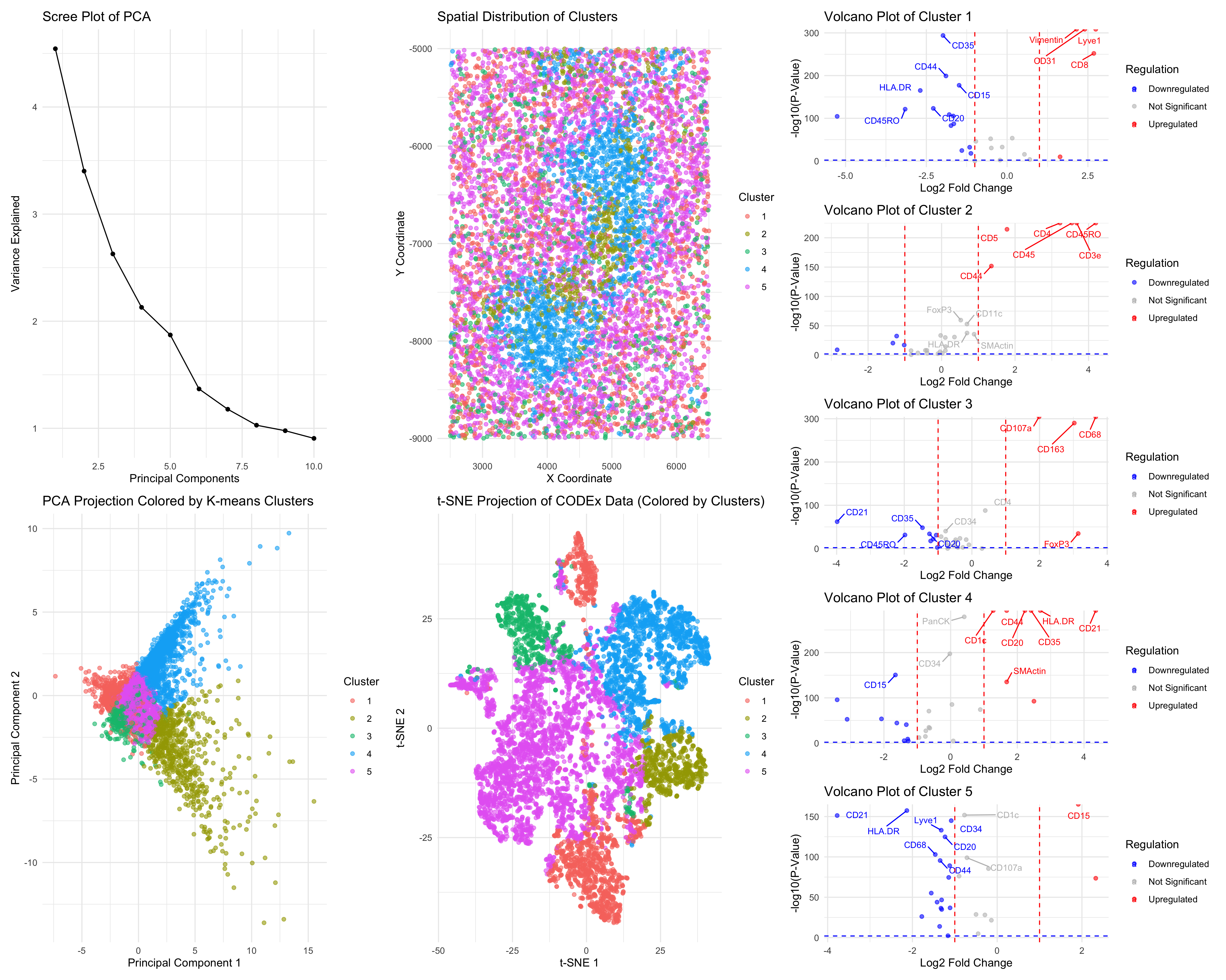
### I think the CODEX dataset represents splenic white pulp. With the available dataset, I have performed log transform, removal of extra data point, K-mean clustering. With those preliminary steps done, I moved on to k=5 clusters and visualize these cluster in PCA, TSNE and spatial physical space. These plots shown distinctive localized cluster, but there are also some areas that are relatively separate out. I was done the wilcoxon two sided test on 5 different clusters and calculate the Log2FC and p-value for genes inside of each cluster to see their significance. With the result got, I visualized them with volcano plot and saw what ever is upregulated and downregulated. Looking at Cluster 2 with key markers of CD3e, CD4 and CD45RO, these are T cells which is the characteristic of the lymphoid tissue in white pulp (Van Krieken, J.H., & te Velde, J.,1986). Looking at cluster 4, the key gene markers are CD21, CD35, and CD20. “These are markers for follicular dendritic cells and B-cells. In mice and rats, the white pulp is composed of Tcell zones, the periarterial lymphatic sheaths (PALSs), and B-cell zones, the follicles and the marginal zone (MZ).” (Steiniger, B.S., 2015). Moreover, Cluster 3 was found to express CD68 and CD163, a marker for marginal zone macrophages that constitute the border of white pulp (Steiniger, B.S., 2015). The distinct cellular populations of the clearly spatially organized tissue in this sample strongly implicate that it is splenic white pulp.
Reference: van Krieken, J. H., & te Velde, J. (1986). Immunohistology of the human spleen: an inventory of the localization of lymphocyte subpopulations. Histopathology, 10(3), 285–294. https://doi.org/10.1111/j.1365-2559.1986.tb02482.x Steiniger B. S. (2015). Human spleen microanatomy: why mice do not suffice. Immunology, 145(3), 334–346. https://doi.org/10.1111/imm.12469 Steiniger B. S. (2015). Human spleen microanatomy: why mice do not suffice. Immunology, 145(3), 334–346. https://doi.org/10.1111/imm.12469
Code (paste your code in between the ``` symbols)
1
2
3
4
5
6
7
8
9
10
11
12
13
14
15
16
17
18
19
20
21
22
23
24
25
26
27
28
29
30
31
32
33
34
35
36
37
38
39
40
41
42
43
44
45
46
47
48
49
50
51
52
53
54
55
56
57
58
59
60
61
62
63
64
65
66
67
68
69
70
71
72
73
74
75
76
77
78
79
80
81
82
83
84
85
86
87
88
89
90
91
92
93
94
95
96
97
98
99
100
101
102
103
104
105
106
107
108
109
110
111
112
113
114
115
116
117
118
119
120
121
122
123
124
125
126
127
128
129
130
131
132
133
134
135
136
137
138
139
140
141
142
143
144
145
146
147
148
149
150
151
152
153
154
155
156
157
158
159
160
161
162
163
164
165
library(ggplot2)
library(Rtsne)
library(dplyr)
library(patchwork)
set.seed(42)
data <- read.csv("/Users/harriethe/GenomicDataVisualization/genomic-data-visualization-2025/data/codex_spleen_3.csv.gz", row.names=1)
head(data)
pos <- data[, c("x", "y")]
exp <- data[, -(1:3)]
exp_norm <- log10(exp + 1)
total_expression <- rowSums(exp_norm)
hist(total_expression, breaks=50, main="Total Expression Distribution", xlab="Total Expression", col="skyblue")
lc_threshold <- quantile(rowSums(data[, -c(1:3)]), 0.25)
data_filtered <- data[rowSums(data[, -c(1:3)]) >= lc_threshold, ]
dim(data)
dim(data_filtered)
#pca
expression_data <- data_filtered[, -c(1:3)]
pcs <- prcomp(expression_data, center = TRUE, scale. = TRUE)
#scree plot
scree_df <- data.frame(PC = 1:length(pcs$sdev), Variance = (pcs$sdev)^2)
scree_plot <- ggplot(scree_df[1:10,], aes(x = PC, y = Variance)) +
  geom_line() +
  geom_point() +
  ggtitle("Scree Plot of PCA") +
  xlab("Principal Components") +
  ylab("Variance Explained") +
  theme_minimal()
print(scree_plot)

ks <- 2:10
wcss <- sapply(ks, function(k) {
  kmeans(pcs$x[, 1:10], centers = k, nstart = 25)$tot.withinss
})
elbow_df <- data.frame(k = ks, WCSS = wcss)
elbow_plot<- ggplot(elbow_df, aes(x = k, y = WCSS)) +
  geom_line() +
  geom_point() +
  theme_minimal() +
  ggtitle("Elbow Method for Optimal k") +
  xlab("Number of Clusters (k)") +
  ylab("Within Cluster Sum of Squares")
# Eh, maybe k=5?
print(elbow_plot)
#scatter plot
pca_df <- data.frame(PC1 = pcs$x[,1], PC2 = pcs$x[,2])
pca_scatter <- ggplot(pca_df, aes(x = PC1, y = PC2)) +
  geom_point(alpha = 0.5) +
  ggtitle("PCA Projection (PC1 vs PC2)") +
  xlab("Principal Component 1") +
  ylab("Principal Component 2") +
  theme_minimal()
print(pca_scatter)

tsne_input <- pcs$x[, 1:10]
set.seed(42)
tsne_result <- Rtsne(tsne_input, perplexity = 30, verbose = TRUE, max_iter = 1000)
tsne_df <- data.frame(tSNE1 = tsne_result$Y[,1], tSNE2 = tsne_result$Y[,2])
library(ggplot2)
ggplot(tsne_df, aes(x = tSNE1, y = tSNE2)) +
  geom_point(alpha = 0.6, color = "blue") +
  theme_minimal() +
  ggtitle("t-SNE Projection of CODEx Data") +
  xlab("t-SNE 1") +
  ylab("t-SNE 2")

#if k = 5
k <- 5
kmeans_result <- kmeans(pcs$x[, 1:10], centers = k, nstart = 25)

# Add cluster labels to the dataset
clusters <- as.factor(kmeans_result$cluster)

# Create PCA scatter plot colored by cluster
pca_cluster_df <- data.frame(PC1 = pcs$x[, 1], PC2 = pcs$x[, 2], Cluster = clusters)

pc_plot <- ggplot(pca_cluster_df, aes(x = PC1, y = PC2, col = Cluster)) +
  geom_point(alpha = 0.6) +
  theme_minimal() +
  ggtitle("PCA Projection Colored by K-means Clusters") +
  xlab("Principal Component 1") +
  ylab("Principal Component 2")
print(pc_plot)

spatial_df <- data.frame(x = data_filtered$x, y = data_filtered$y, Cluster = clusters)

spatial_plot <- ggplot(spatial_df, aes(x = x, y = y, col = Cluster)) +
  geom_point(alpha = 0.6) +
  theme_minimal() +
  ggtitle("Spatial Distribution of Clusters") +
  xlab("X Coordinate") +
  ylab("Y Coordinate")
print(spatial_plot)

# tsne cluster

tsne_df$Cluster <- as.factor(clusters)
tsne_plot <- ggplot(tsne_df, aes(x = tSNE1, y = tSNE2, color = Cluster)) +
  geom_point(alpha = 0.6) +
  theme_minimal() +
  ggtitle("t-SNE Projection of CODEx Data (Colored by Clusters)") +
  xlab("t-SNE 1") +
  ylab("t-SNE 2")

print(tsne_plot)
#calculate wilcoxon test
de_results <- list()
for (i in levels(clusters)) {
  cluster_cells <- names(clusters)[clusters == i]
  other_cells <- names(clusters)[clusters != i]

  p_values <- apply(data_filtered[, -c(1:3)], 2, function(gene) {
    wilcox.test(gene[cluster_cells], gene[other_cells], alternative = 'two.sided')$p.value
  })

  log2FC <- apply(data_filtered[, -c(1:3)], 2, function(gene) {
    mean_cluster <- mean(gene[cluster_cells])
    mean_other <- mean(gene[other_cells])
    log2(mean_cluster / mean_other)
  })

  de_results[[i]] <- data.frame(Gene = names(p_values), Log2FC = log2FC, P_Value = p_values) %>%
    arrange(P_Value) %>%
    mutate(Cluster = i)
}

de_markers <- bind_rows(de_results)
de_markers <- de_markers %>%
  mutate(Significant = ifelse(P_Value < 0.01 & abs(Log2FC) > 1, "Yes", "No"))
top_markers <- de_markers %>%
  filter(Significant == "Yes") %>%
  group_by(Cluster) %>%
  slice_min(P_Value, n = 10)
volcano_plots <- list()
unique_clusters <- unique(de_markers$Cluster)
for (cl in unique_clusters) {
  cluster_data <- subset(de_markers, Cluster == cl)
  cluster_data$Regulation <- ifelse(cluster_data$Log2FC > 1 & cluster_data$P_Value < 0.01, "Upregulated",
                             ifelse(cluster_data$Log2FC < -1 & cluster_data$P_Value < 0.01, "Downregulated", "Not Significant"))
  top_genes <- cluster_data[order(cluster_data$P_Value), ][1:10, ]


  volcano_plot <- ggplot(cluster_data, aes(x = Log2FC, y = -log10(P_Value), col = Regulation)) +
    geom_point(alpha = 0.6) +
    scale_color_manual(values = c("Upregulated" = "red", "Downregulated" = "blue", "Not Significant" = "gray")) +
    theme_minimal() +
    ggtitle(paste("Volcano Plot of Cluster", cl)) +
    xlab("Log2 Fold Change") +
    ylab("-log10(P-Value)") +
    geom_hline(yintercept = -log10(0.01), linetype = "dashed", color = "blue") +
    geom_vline(xintercept = c(-1, 1), linetype = "dashed", color = "red") +
    geom_text_repel(data = top_genes, aes(label = Gene, col = Regulation), size = 3, box.padding = 0.5, max.overlaps = 15)
  volcano_plots[[paste0("volcano_cluster", cl)]] <- volcano_plot
}
names(volcano_plots)

final_plot <- (scree_plot / pc_plot) | (spatial_plot / tsne_plot) |
              (volcano_plots$volcano_cluster1 /
               volcano_plots$volcano_cluster2  /
               volcano_plots$volcano_cluster3 /
               volcano_plots$volcano_cluster4  /
               volcano_plots$volcano_cluster5)
png("hw5_jhe46.png", width = 5000, height = 4000, res = 300)
print(final_plot)
dev.off()