Clustering and Spatial Analysis of CODEX Tissue Types

Identifying White Pulp and Structural Fibroblast Populations in the Spleen
To classify the tissue type in the CODEX dataset, I first applied log transformation and normalization to the protein expression data to ensure comparability across cells. I then performed PCA, followed by t-SNE for visualization. Using k-means clustering, I grouped cells into k=8 distinct clusters and performed differential expression analysis to identify significantly upregulated proteins.
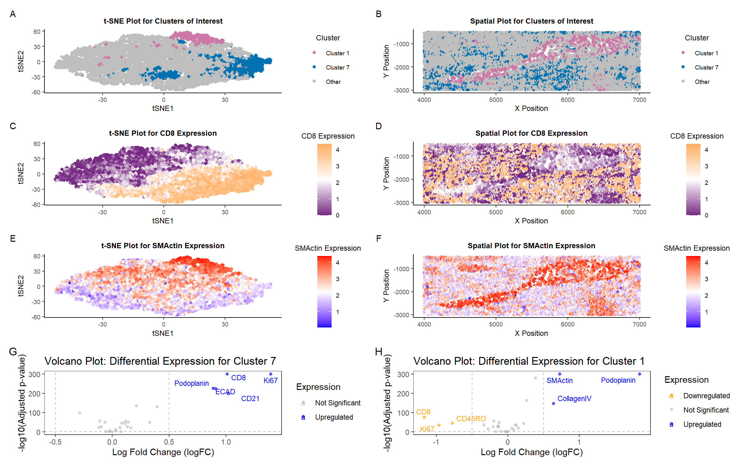
To determine the biological identity of these clusters, I conducted Wilcoxon tests to identify the most significantly upregulated proteins in Clusters 7 and 1. I prioritized those with the smallest p-values to ensure strong statistical support. Cluster 7 exhibited a high expression of CD8, which indicates a predominance of cytotoxic T cells1. Cluster 1 showed strong upregulation of SMActin, suggesting a population of smooth muscle cells2. I examined them in t-SNE space (plot A) and in tissue space (plot B). Additionally, I mapped CD8 and SMActin to further explore their significance in distinguishing tissue structures.
In Cluster 7, the most significantly upregulated proteins include CD8, Ki67, CD21, and Podoplanin (plot G). CD8 and Ki67 are hallmark markers of active T cells, suggesting that this cluster is rich in cytotoxic T lymphocytes (CTLs) undergoing proliferation3. CD21 is associated with follicular dendritic cells and B-cell zones4. These are known to be key components of the white pulp5. The presence of Podoplanin, which is involved in stromal-immune crosstalk, further reinforces this classification6. These markers strongly indicate that Cluster 7 represents the white pulp, where adaptive immune responses occur.
In contrast, Cluster 1 exhibits high expression of SMActin, Collagen IV, and Podoplanin, all structural proteins associated with mesenchymal and stromal cells (plot H). SMActin (smooth muscle actin) is a marker of contractile fibroblasts, which are abundant in the spleen’s capsule and trabeculae5,7. Additionally, Collagen IV is a major structural component of the extracellular matrix of the basement membrane of the spleen8. The downregulation of immune-related markers such as CD8, Ki67, and CD45RO suggests that this region is less involved in immune cell activation compared to white pulp. Given the predominance of fibrous structural proteins and the lack of immune activity, Cluster 1 likely corresponds to the capsule or trabeculae, providing mechanical support and structural integrity to the spleen.
To further support these classifications, I examined the expression of a highly upregulated protein from each cluster in both t-SNE space and tissue space. Mapping CD8 and SMActin, which are strongly upregulated in Clusters 7 and 1, respectively, revealed a clear separation: CD8 was highly concentrated in Cluster 7 in t-SNE space (plot C), reinforcing its role in white pulp immune function, whereas SMActin was localized to Cluster 1 (plot E), reinforcing its role in the fibrous support network. This spatial organization aligns with known spleen architecture, where the capsule and trabeculae (plot F) form a protective framework, while the white pulp (plot D) is the primary site of adaptive immune responses5.
Interestingly, Podoplanin is upregulated in both Clusters 7 and 1, yet its co-expressed markers differ, highlighting distinct tissue roles. In Cluster 7, Podoplanin appears alongside immune markers (CD8, Ki67), suggesting involvement in lymphoid structure organization. In Cluster 1, it is co-expressed with fibrous structural proteins (SMActin, Collagen IV), reinforcing its role in the capsule or trabeculae5. This difference highlights the importance of considering marker co-expression rather than single-marker presence when classifying tissue identity.
Based on these expression patterns and spatial organization, the high presence of CD8+ T cells in Cluster 7 corresponds to the immune-active white pulp. In Cluster 1, the predominance of SMActin-expressing fibroblasts aligns with the structural capsule or trabeculae. These classifications are consistent with known spleen microanatomy.
References
- https://www.ncbi.nlm.nih.gov/gene/925
- https://www.researchgate.net/figure/SMACTIN-smooth-muscle-actin-paraffin-cross-section-from-POEMS-a-and-CIDP-b_fig2_309595968
- https://www.nature.com/articles/s41392-023-01471-y#:~:text=In%20the%20acute%20phase%20of,%2C%20perforin%2C%20and%20granzyme%20B.
- https://www.neobiotechnologies.com/resources/cd21-b-cell/#:~:text=In%20our%20exploration%20of%20B,activation%2C%20proliferation%2C%20and%20survival.
- https://journals.sagepub.com/doi/10.1080/01926230600867743?url_ver=Z39.88-2003&rfr_id=ori:rid:crossref.org&rfr_dat=cr_pub%20%200pubmed
- https://www.nature.com/articles/s41577-025-01140-x
- https://www.molbiolcell.org/doi/full/10.1091/mbc.12.9.2730
- https://www.sciencedirect.com/science/article/pii/S1044532307001157
# import libraries
library(here)
library(ggplot2)
library(Rtsne)
library(patchwork)
library(factoextra)
library(ggrepel)
library(viridis)
library(scales)


# read in data
data <- read.csv('codex_spleen_subset.csv.gz', row.names=1)


# extract data.  there are 2 position columns, 1 area column, and  28 expression-related columns
pos <- data[, 1:2]
area <- data[, 3]
pexp <- data[, 4:31]


# normalize
pexpnorm <- log10(pexp/rowSums(pexp) * mean(rowSums(pexp)) + 1)
names(pexpnorm)


# perform pca
pcs <- prcomp(pexpnorm)
plot(pcs$sdev, main = "Scree Plot", xlab = "Principal Components", ylab = "Standard Deviation")


# perform tsne on top PCs
set.seed(02242025)
emb <- Rtsne(pcs$x[, 1:10], perplexity = 15)


# find optimal k using Elbow Method
fviz_nbclust(data.frame(pcs$x[, 1:10]), kmeans, method = "wss")


# use quantitative variable k = 8 clusters
k = 8


# perform kmeans clustering based on elbow plot
clusters <- as.factor(kmeans(pcs$x[, 1:10], centers = k)$cluster)
df_clusters <- data.frame(pcs$x)
df_clusters$cluster <- clusters
df_pca <- data.frame(PC1 = pcs$x[,1], PC2 = pcs$x[,2], Cluster = clusters)
df_tsne <- data.frame(tSNE1 = emb$Y[,1], tSNE2 = emb$Y[,2], Cluster = clusters)


# focus on clusters 7 and 1
first_cluster <- 7
second_cluster <- 1


# single the clusters of interest out
cluster_of_interest <- ifelse(clusters == first_cluster, paste("Cluster", first_cluster),
                              ifelse(clusters == second_cluster, paste("Cluster", second_cluster), "Other"))

df_clusters$highlight <- ifelse(clusters == first_cluster, paste("Cluster", first_cluster),
                                ifelse(clusters == second_cluster, paste("Cluster", second_cluster), "Other"))

# pca scatter plot by clusters
pca_plot <- ggplot(df_pca, aes(x = PC1, y = PC2, color = Cluster)) +
  geom_point(size=1) +
  theme_bw() +
  labs(title = "PCA Plot colored by Clusters", color = "Cluster", x = "PC1", y = "PC2") +
  theme(legend.title.align=0.5, plot.title = element_text(hjust = 0.5, face="bold", size=9), text = element_text(size = 8)) +
  guides(color = guide_legend(override.aes = list(size=4)))


# tsne scatter plot with clusters
tsne_plot <- ggplot(df_tsne, aes(x = tSNE1, y = tSNE2, color = Cluster)) +
  geom_point(size=1.75) +
  theme_bw() +
  labs(title = "t-SNE Plot colored by Clusters", color = "Cluster", x = "tSNE1", y = "tSNE2") +
  theme(legend.title.align=0.5, plot.title = element_text(hjust = 0.5, face="bold", size=9), text = element_text(size = 9)) +
  guides(color = guide_legend(override.aes = list(size=4)))


# tsne scatter plot singling out clusters of interest
first_cluster_label <- paste("Cluster", first_cluster)
second_cluster_label <- paste("Cluster", second_cluster)

p1 <- ggplot(data.frame(emb$Y, cluster_of_interest)) +
  geom_point(aes(x = emb$Y[,1], y = emb$Y[,2], color = cluster_of_interest), size=1.5) +
  scale_color_manual(
    name = "Cluster",
    values = setNames(c("#0072B2",  # Blue for first cluster
                        "#CC79A7",  # Dark Pink for second cluster
                        "gray"),    # Gray for other clusters
                      c(first_cluster_label, second_cluster_label, "Other"))) +
  theme_classic() +
  labs(title = "t-SNE Plot for Clusters of Interest",
       x = "tSNE1",
       y = "tSNE2") +
  theme(legend.title.align=0.5,
        plot.title = element_text(hjust = 0.5, face="bold", size=9),
        text = element_text(size = 9))


# differential expression analysis on first cluster
pv <- sapply(colnames(pexpnorm), function(i) {
  print(i)
  wilcox.test(pexpnorm[clusters == first_cluster, i], pexpnorm[clusters != first_cluster, i])$p.val
})

logfc <- sapply(colnames(pexpnorm), function(i) {
  print(i)
  log2(mean(pexpnorm[clusters == first_cluster, i])/mean(pexpnorm[clusters != first_cluster, i]))
})

# create a dataframe for first Volcano plot, adjusting and converting p-values
df_volcano <- data.frame(Gene = colnames(pexpnorm), p_value = pv, logFC = logfc)
df_volcano$adj_p_value <- p.adjust(df_volcano$p_value, method = "fdr")
df_volcano$logP <- -log10(df_volcano$adj_p_value + 1e-300)

# define Upregulated and Downregulated Genes
df_volcano$Expression <- "Not Significant"
df_volcano$Expression[df_volcano$logFC > 0.5 & df_volcano$adj_p_value < 0.05] <- "Upregulated"
df_volcano$Expression[df_volcano$logFC < -0.5 & df_volcano$adj_p_value < 0.05] <- "Downregulated"
df_volcano <- df_volcano[complete.cases(df_volcano), ]   # Remove rows with NA values
df_volcano <- df_volcano[is.finite(df_volcano$logFC) & is.finite(df_volcano$logP), ]   # Remove Inf values

top_up <- df_volcano[df_volcano$Expression == "Upregulated", ]
if (nrow(top_up) > 5) {
  top_up <- top_up[order(top_up$p_value), ][1:5, ]  # Sort by p-value (ascending) and select top 5
} else {
  top_up <- top_up  # If fewer than 5, keep all available upregulated genes
}

top_down <- df_volcano[df_volcano$Expression == "Downregulated", ]
if (nrow(top_down) > 5) {
  top_down <- top_down[order(top_down$p_value), ][1:5, ]
} else {
  top_down <- top_down  # Keep all available downregulated genes if <5
}

# first Volcano plot
v1 <- ggplot(df_volcano, aes(x = logFC, y = logP, color = Expression)) +
  geom_point(alpha = 0.6) +
  geom_text_repel(data = top_up, aes(label = Gene), size = 3) +
  geom_text_repel(data = top_down, aes(label = Gene), size = 3) +
  geom_text_repel(data = df_volcano[df_volcano$Gene == "CD79A", ],
                  aes(label = Gene), size = 4, color = "darkblue", fontface = "bold", nudge_x=1, nudge_y=20) +
  scale_color_manual(values = c("Upregulated" = "blue",
                                "Not Significant" = "grey",
                                "Downregulated" = "orange")) +
  labs(title = paste0("Volcano Plot: Differential Expression for Cluster ", first_cluster),
       x = "Log Fold Change (logFC)",
       y = "-log10(Adjusted p-value)") +
  geom_hline(yintercept = -log10(0.05), linetype = "dashed", color = "grey") +
  geom_vline(xintercept = c(-0.5, 0.5), linetype = "dashed", color = "grey") +
  theme(plot.title = element_text(size = 7)) +
  theme_bw() +
  theme(panel.grid.major = element_blank(), panel.grid.minor = element_blank())


# differential expression analysis on second cluster
pv2 <- sapply(colnames(pexpnorm), function(i) {
  print(i)
  wilcox.test(pexpnorm[clusters %in% second_cluster, i], pexpnorm[!clusters %in% second_cluster, i])$p.val
})

logfc2 <- sapply(colnames(pexpnorm), function(i) {
  print(i)
  log2(mean(pexpnorm[clusters %in% second_cluster, i])/mean(pexpnorm[!clusters %in% second_cluster, i]))
})

# create a dataframe for second Volcano plot, adjusting and converting p-values
df_volcano2 <- data.frame(Gene = colnames(pexpnorm), p_value = pv2, logFC = logfc2)
df_volcano2$adj_p_value <- p.adjust(df_volcano2$p_value, method = "fdr")
df_volcano2$logP <- -log10(df_volcano2$adj_p_value + 1e-300)

# define Upregulated and Downregulated Genes
df_volcano2$Expression <- "Not Significant"
df_volcano2$Expression[df_volcano2$logFC > 0.5 & df_volcano2$adj_p_value < 0.05] <- "Upregulated"
df_volcano2$Expression[df_volcano2$logFC < -0.5 & df_volcano2$adj_p_value < 0.05] <- "Downregulated"
df_volcano2 <- df_volcano2[complete.cases(df_volcano2), ]   # Remove rows with NA values
df_volcano2 <- df_volcano2[is.finite(df_volcano2$logFC) & is.finite(df_volcano2$logP), ]   # Remove Inf values

top_up2 <- df_volcano2[df_volcano2$Expression == "Upregulated", ]
if (nrow(top_up2) > 5) {
  top_up2 <- top_up2[order(top_up2$p_value), ][1:5, ]  # Sort by p-value (ascending) and select top 5
} else {
  top_up2 <- top_up2  # If fewer than 5, keep all available upregulated genes
}

top_down2 <- df_volcano2[df_volcano2$Expression == "Downregulated", ]
if (nrow(top_down2) > 5) {
  top_down2 <- top_down2[order(top_down2$p_value), ][1:5, ]
} else {
  top_down2 <- top_down2  # Keep all available downregulated genes if <5
}

# second Volcano plot
v2 <- ggplot(df_volcano2, aes(x = logFC, y = logP, color = Expression)) +
  geom_point(alpha = 0.6) +
  geom_text_repel(data = top_up2, aes(label = Gene), size = 3) +
  geom_text_repel(data = top_down2, aes(label = Gene), size = 3) +
  scale_color_manual(values = c("Upregulated" = "blue",
                                "Not Significant" = "grey",
                                "Downregulated" = "orange")) +
  labs(title = paste0("Volcano Plot: Differential Expression for Cluster ", second_cluster),
       x = "Log Fold Change (logFC)",
       y = "-log10(Adjusted p-value)") +
  geom_hline(yintercept = -log10(0.05), linetype = "dashed", color = "grey") +
  geom_vline(xintercept = c(-0.5, 0.5), linetype = "dashed", color = "grey") +
  theme(plot.title = element_text(size = 7)) +
  theme_bw() +
  theme(panel.grid.major = element_blank(), panel.grid.minor = element_blank())

print(top_up)
print(top_down)
print(top_up2)
print(top_down2)


# Spatial plot for clusters of interest
df_clusters$x <- pos$x
df_clusters$y <- pos$y
df_clusters$cluster_of_interest <- ifelse(clusters == first_cluster, paste("Cluster", first_cluster), "Other")
df_clusters$cluster_of_interest <- ifelse(clusters == second_cluster, paste("Cluster", second_cluster), df_clusters$cluster_of_interest)
df_clusters$cluster_of_interest <- as.factor(df_clusters$cluster_of_interest)

p2 <- ggplot(df_clusters) +
  geom_point(aes(x = x, y = y, color = cluster_of_interest), size = 1.5) +
  #scale_color_manual(name = "Cluster", values = c("Cluster 4" = "#0072B2", "Cluster 8" = "#CC79A7", "Other" = "gray")) +
  scale_color_manual(
    name = "Cluster",
    values = setNames(c("#0072B2",  # Blue for first cluster
                        "#CC79A7",  # Dark Pink for second cluster
                        "gray"),    # Gray for other clusters
                      c(first_cluster_label, second_cluster_label, "Other"))) +
  theme_classic() +
  labs(
    title = "Spatial Plot for Clusters of Interest", x = "X Position", y = "Y Position") +
  theme(
    legend.title.align=0.5, plot.title = element_text(hjust=0.5, face="bold", size=9), text=element_text(size=9))


# assign CD8 expression values
df_clusters$CD8_expr <- pexpnorm$CD8

# t-SNE plot for CD8 Expression
c1 <- ggplot(data.frame(emb$Y, CD8_expr = pexpnorm$CD8)) +
  geom_point(aes(x = emb$Y[,1], y = emb$Y[,2], color = CD8_expr), size=1.5) +
  #scale_color_gradientn(colors = c("#D3D3D3", "#9370DB", "#4B0082")) +
  scale_color_gradientn(colors = c("#762A83", "white", "#FFAD60")) +
  theme_classic() +
  labs(title = "t-SNE Plot for CD8 Expression", color = "CD8 Expression", x = "tSNE1", y = "tSNE2") +
  theme(legend.title.align=0.5, plot.title = element_text(hjust = 0.5, face="bold", size=9), text = element_text(size=9))


# Spatial plot for CD8 Expression
c2 <- ggplot(df_clusters) +
  geom_point(aes(x = x, y = y, color = CD8_expr), size = 1.5) +
  scale_color_gradientn(colors = c("#762A83", "white", "#FFAD60")) +
  theme_classic() +
  labs(title = "Spatial Plot for CD8 Expression", color = "CD8 Expression", x = "X Position", y = "Y Position") +
  theme(legend.title.align=0.5, plot.title=element_text(hjust=0.5, face="bold", size=9), text=element_text(size=9))


# assign SMActin expression values
df_clusters$SMActin_expr <- pexpnorm$SMActin

# t-SNE Plot for SMActin Expression
s1 <- ggplot(data.frame(emb$Y, SMActin_expr = pexpnorm$SMActin)) +
  geom_point(aes(x = emb$Y[,1], y = emb$Y[,2], color = SMActin_expr), size=1.5) +
  scale_color_gradientn(colors = c("blue", "white", "red")) +
  theme_classic() +
  labs(title = "t-SNE Plot for SMActin Expression", color = "SMActin Expression", x = "tSNE1", y = "tSNE2") +
  theme(legend.title.align=0.5, plot.title = element_text(hjust = 0.5, face="bold", size=9), text = element_text(size=9))


# Spatial Plot for SMActin Expression
s2 <- ggplot(df_clusters) +
  geom_point(aes(x = x, y = y, color = SMActin_expr), size = 1.5) +
  scale_color_gradientn(colors = c("blue", "white", "red")) +
  theme_classic() +
  labs(title = "Spatial Plot for SMActin Expression", color = "SMActin Expression", x = "X Position", y = "Y Position") +
  theme(legend.title.align=0.5, plot.title=element_text(hjust=0.5, face="bold", size=9), text=element_text(size=9))


# plot using patchwork
p1 + p2 + c1 + c2 + s1 + s2 + v1 + v2  + plot_annotation(tag_levels = 'A') + plot_layout(nrow = 4, ncol = 2)