Analyzing Immune Cell Clusters in CODEX Dataset

I'm a junior at Johns Hopkins.

Analyzing Immune Cell Clusters in CODEX Dataset

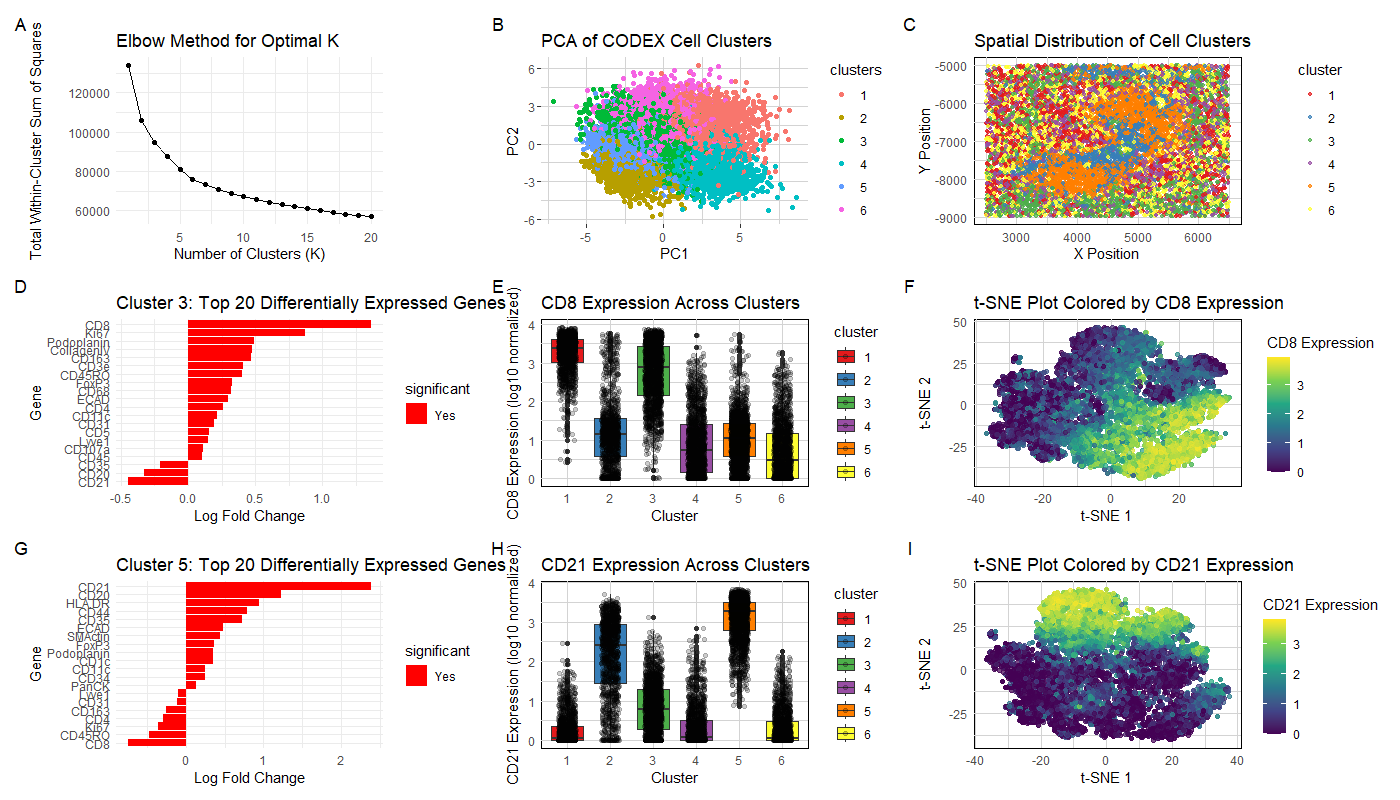
Visualization Summary In this visualization, I analyzed two cell types within the CODEX dataset: T cells and B cells. First, the genes in the dataset were normalized, log-transformed, and clustered (K = 6). The ideal K was determined through plotting the total-withiness scores for K = [1, 20]. Then, based on the elbow method heuristic, the optimal number of clusters was determined to be 6 (Figure A). To understand gene clustering and expression similarity profiles, and to reduce the dimensionality of the dataset, principal component analysis was performed (Figure B). A spatial analysis of the clusters was also visualized (Figure C). Clusters 3 and 5 were chosen for further investigation and differential gene expression analysis was performed on both clusters. A CD8 phenotype was identified in Cluster 3 (shown by Figure E, F), and a CD21 phenotype was identified in Cluster 5 (Figure H, I).

CD8 has long been classified as having a cytotoxic T cell phenotype [1], and CD21 (combined with CD20) which were both highly differentially expressed are associated with B cells [2]. Due to the discovery of these cell phenotypes, the CODEX dataset contains white pulp tissue which refers to lymphatic tissue (i.e., produces lymphocytes) [3]. Both T cells and B cells are lymphocytes.

References: [1] Koh, C. H., Lee, S., Kwak, M., Kim, B. S., & Chung, Y. (2023). CD8 T-cell subsets: heterogeneity, functions, and therapeutic potential. Experimental & molecular medicine, 55(11), 2287–2299. https://doi.org/10.1038/s12276-023-01105-x [2] Rahe, M. C., Dvorak, C. M. T., Wiseman, B., Martin, D., & Murtaugh, M. P. (2020). Establishment and characterization of a porcine B cell lymphoma cell line. Experimental cell research, 390(2), 111986. https://doi.org/10.1016/j.yexcr.2020.111986 [3] Lewis, S. M., Williams, A., & Eisenbarth, S. C. (2019). Structure and function of the immune system in the spleen. Science immunology, 4(33), eaau6085. https://doi.org/10.1126/sciimmunol.aau6085

Code (paste your code in between the ``` symbols)

library(ggplot2)
library(dplyr)
library(tidyr)
library(RColorBrewer)
library(patchwork)
library(Rtsne)

file <- 'codex_spleen_3.csv.gz'
data <- read.csv(file)
data[1:5,1:10]

## K Means Clustering + Principal Component Analysis
pos <- data[, 2:3]
rownames(pos) <- data$cell_id
gexp <- data[, 5:ncol(data)]
rownames(gexp) <- data$barcode
gene_norm <- log10(gexp * 10000 / rowSums(gexp) + 1)

# Compute Total Withiness
compute_wcss <- function(data, k) {
  km <- kmeans(data, centers = k, nstart = 10)
  return(km$tot.withinss)
}

# Compute WCSS for a range of K values
k_values <- 1:20  # You can adjust this range as needed
wcss_values <- sapply(k_values, function(k) compute_wcss(gene_norm, k))

# Create a data frame for plotting
elbow_data <- data.frame(K = k_values, WCSS = wcss_values)

# Plot the elbow curve
elbow_plot <- ggplot(elbow_data, aes(x = K, y = WCSS)) +
  geom_line() +
  geom_point() +
  labs(title = "Elbow Method for Optimal K",
       x = "Number of Clusters (K)",
       y = "Total Within-Cluster Sum of Squares") +
  theme_minimal()

print(elbow_plot)

# K Means Clustering 
com <- kmeans(gene_norm, centers=6)
clusters <- com$cluster
clusters <- as.factor(clusters)
names(clusters) <- rownames(gene_norm)
head(clusters)

pca_result <- prcomp(gene_norm, scale. = TRUE)
summary(pca_result)

df <- data.frame(pca_result$x, clusters)
p1 <- ggplot(df, aes(x = PC1, y = PC2, col = clusters)) +
  geom_point() +
  labs(title = "PCA of CODEX Cell Clusters") +
  theme(
    panel.background = element_rect(fill = "white"),
    panel.grid.major = element_line(color = "lightgray"),
    panel.grid.minor = element_line(color = "lightgray")
  )

print(p1)

# Combine position data with cluster information
spatial_data <- data.frame(pos, cluster = clusters)

# Create a spatial plot
p2 <- ggplot(spatial_data, aes(x = x, y = y, color = cluster)) +
  geom_point(size = 1, alpha = 0.7) +
  scale_color_brewer(palette = "Set1") +
  labs(title = "Spatial Distribution of Cell Clusters",
       x = "X Position", y = "Y Position") +
  theme_minimal() +
  theme(
    panel.background = element_rect(fill = "white"),
    panel.grid.major = element_line(color = "lightgray"),
    panel.grid.minor = element_line(color = "lightgray")
  )

print(p2)

# Differential Gene Expression Cluster 3

# Create a binary vector for cluster 3 vs others
cluster3_vs_others <- ifelse(clusters == 3, 1, 0)

# Function to perform t-test for each gene
perform_t_test <- function(gene) {
  test_result <- t.test(gene_norm[cluster3_vs_others == 1, gene], 
                        gene_norm[cluster3_vs_others == 0, gene])
  return(c(p_value = test_result$p.value, 
           t_statistic = test_result$statistic))
}

# Perform t-test for all genes
t_test_results <- t(sapply(colnames(gene_norm), perform_t_test))

# Calculate log fold change
log_fc <- sapply(colnames(gene_norm), function(gene) {
  mean(gene_norm[cluster3_vs_others == 1, gene]) - 
    mean(gene_norm[cluster3_vs_others == 0, gene])
})

# Combine results
results <- data.frame(
  gene = colnames(gene_norm),
  log_fc = log_fc,
  p_value = t_test_results[, "p_value"],
  t_statistic = t_test_results[, "t_statistic.t"]
)

# Adjust p-values for multiple testing
results$adj_p_value <- p.adjust(results$p_value, method = "BH")

# Sort by adjusted p-value
results <- results[order(results$adj_p_value), ]

# Add significance column
results$significant <- ifelse(results$adj_p_value < 0.05, "Yes", "No")
top_genes <- head(results, 20)

p4 <- ggplot(top_genes, aes(x = reorder(gene, log_fc), y = log_fc, fill = significant)) +
  geom_bar(stat = "identity") +
  scale_fill_manual(values = c("No" = "grey", "Yes" = "red")) +
  coord_flip() +
  labs(title = "Cluster 3: Top 20 Differentially Expressed Genes",
       x = "Gene",
       y = "Log Fold Change") +
  theme_minimal()

print(p4)

## Check if CD8 is unique to cluster 3
# Create a data frame with CD8 expression and cluster information
cd8_data <- data.frame(CD8 = gene_norm[, "CD8"], cluster = clusters)

# Calculate mean CD8 expression for each cluster
cd8_mean <- cd8_data %>%
  group_by(cluster) %>%
  summarise(mean_expression = mean(CD8))

# Create a box plot
p_cd8 <- ggplot(cd8_data, aes(x = cluster, y = CD8, fill = cluster)) +
  geom_boxplot() +
  geom_jitter(width = 0.2, alpha = 0.2) +
  scale_fill_brewer(palette = "Set1") +
  labs(title = "CD8 Expression Across Clusters",
       x = "Cluster",
       y = "CD8 Expression (log10 normalized)") +
  theme_minimal() +
  theme(
    panel.background = element_rect(fill = "white"),
    panel.grid.major = element_line(color = "lightgray"),
    panel.grid.minor = element_line(color = "lightgray")
  )

print(p_cd8)

# Perform t-SNE
set.seed(42)  # for reproducibility
tsne_result <- Rtsne(gene_norm, dims = 2, perplexity = 30, verbose = TRUE, max_iter = 1000)

# Create a data frame with t-SNE results and CD8 expression
tsne_df <- data.frame(
  tSNE1 = tsne_result$Y[,1],
  tSNE2 = tsne_result$Y[,2],
  CD8 = gene_norm[, "CD8"]
)

# Create the t-SNE plot
p_tsne_cd8 <- ggplot(tsne_df, aes(x = tSNE1, y = tSNE2, color = CD8)) +
  geom_point(alpha = 0.7) +
  scale_color_viridis_c() +
  labs(title = "t-SNE Plot Colored by CD8 Expression",
       x = "t-SNE 1",
       y = "t-SNE 2",
       color = "CD8 Expression") +
  theme_minimal() +
  theme(
    panel.background = element_rect(fill = "white"),
    panel.grid.major = element_line(color = "lightgray"),
    panel.grid.minor = element_line(color = "lightgray")
  )

print(p_tsne_cd8)

##############################

# Differential Gene Expression Cluster 5

# Create a binary vector for cluster 5 vs others
cluster5_vs_others <- ifelse(clusters == 5, 1, 0)

# Function to perform t-test for each gene
perform_t_test <- function(gene) {
  test_result <- t.test(gene_norm[cluster5_vs_others == 1, gene], 
                        gene_norm[cluster5_vs_others == 0, gene])
  return(c(p_value = test_result$p.value, 
           t_statistic = test_result$statistic))
}

# Perform t-test for all genes
t_test_results <- t(sapply(colnames(gene_norm), perform_t_test))

# Calculate log fold change
log_fc <- sapply(colnames(gene_norm), function(gene) {
  mean(gene_norm[cluster5_vs_others == 1, gene]) - 
    mean(gene_norm[cluster5_vs_others == 0, gene])
})

# Combine results
results <- data.frame(
  gene = colnames(gene_norm),
  log_fc = log_fc,
  p_value = t_test_results[, "p_value"],
  t_statistic = t_test_results[, "t_statistic.t"]
)

# Adjust p-values for multiple testing
results$adj_p_value <- p.adjust(results$p_value, method = "BH")

# Sort by adjusted p-value
results <- results[order(results$adj_p_value), ]

# Add significance column
results$significant <- ifelse(results$adj_p_value < 0.05, "Yes", "No")
top_genes <- head(results, 20)

p5 <- ggplot(top_genes, aes(x = reorder(gene, log_fc), y = log_fc, fill = significant)) +
  geom_bar(stat = "identity") +
  scale_fill_manual(values = c("No" = "grey", "Yes" = "red")) +
  coord_flip() +
  labs(title = "Cluster 5: Top 20 Differentially Expressed Genes",
       x = "Gene",
       y = "Log Fold Change") +
  theme_minimal()

print(p5)

## CD21 Analysis
cd21_data <- data.frame(CD21 = gene_norm[, "CD21"], cluster = clusters)

# Calculate mean CD8 expression for each cluster
cd21_mean <- cd21_data %>%
  group_by(cluster) %>%
  summarise(mean_expression = mean(CD21))

# Create a box plot
p_cd21 <- ggplot(cd21_data, aes(x = cluster, y = CD21, fill = cluster)) +
  geom_boxplot() +
  geom_jitter(width = 0.2, alpha = 0.2) +
  scale_fill_brewer(palette = "Set1") +
  labs(title = "CD21 Expression Across Clusters",
       x = "Cluster",
       y = "CD21 Expression (log10 normalized)") +
  theme_minimal() +
  theme(
    panel.background = element_rect(fill = "white"),
    panel.grid.major = element_line(color = "lightgray"),
    panel.grid.minor = element_line(color = "lightgray")
  )

print(p_cd21)

# Perform t-SNE for CD21
set.seed(42)  # for reproducibility
tsne_result <- Rtsne(gene_norm, dims = 2, perplexity = 30, verbose = TRUE, max_iter = 1000)

# Create a data frame with t-SNE results and CD8 expression
tsne_df <- data.frame(
  tSNE1 = tsne_result$Y[,1],
  tSNE2 = tsne_result$Y[,2],
  CD21 = gene_norm[, "CD21"]
)

# Create the t-SNE plot
p_tsne_cd21 <- ggplot(tsne_df, aes(x = tSNE1, y = tSNE2, color = CD21)) +
  geom_point(alpha = 0.7) +
  scale_color_viridis_c() +
  labs(title = "t-SNE Plot Colored by CD21 Expression",
       x = "t-SNE 1",
       y = "t-SNE 2",
       color = "CD21 Expression") +
  theme_minimal() +
  theme(
    panel.background = element_rect(fill = "white"),
    panel.grid.major = element_line(color = "lightgray"),
    panel.grid.minor = element_line(color = "lightgray")
  )

print(p_tsne_cd21)

## Make combined plot
combined_plot <- (elbow_plot + p1 + p2 + p4 + p_cd8 + p_tsne_cd8 + p5 + p_cd21 + p_tsne_cd21) + plot_layout(ncol = 3) +
  plot_annotation(tag_levels = 'A')

print(combined_plot)

ggsave("hw5_sraghav9_v1.png", combined_plot, width = 18, height = 10, units = "in", dpi = 300)

27 Feb 2025

« Identifying tissue structure in spleen tissue sample Analysis of CODEX dataset »