Identifying White Pulp Tissue Structure in CODEX Data

1. Figure Description and Interpretation
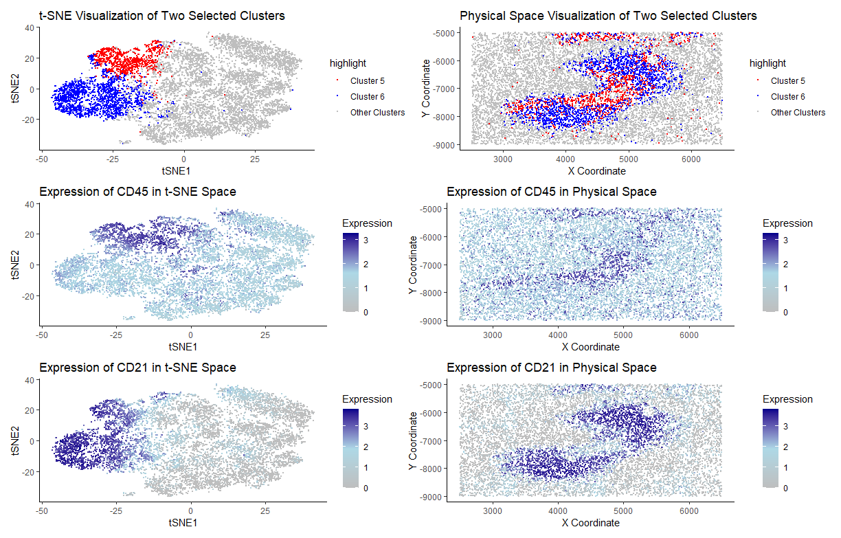
I have performed quality control, dimensionality reduction using t-SNE, k-means clustering with optimal k=9 (from an elbow plot), and differential expression analysis on the CODEX data. Based on the spatial patterns both in the tSNE cluster plot and physical space cluster plot, I choose to focus on Clusters 5 and 6. The figures on the first row visualize these clusters both in the tSNE space and physical space. It’s clear to see that both clusters have distinct patterns in the tSNE space, while they mix together in the middle region in the physical space. Based on differential gene expression analysis, I found out CD45 is differentially expressed in Cluster 5, while CD21 is differentially expressed in Cluster 6. Figures on row 2 illustrate the expression pattern for CD45 - up-regulated in Cluster 5 both in t-SNE and physical space. Similar patterns could be seen for figures on row 3, which illustrate the expression pattern for CD21 in Cluster 6.
Based on my analysis, I choose to focus on CD21 and CD45. Based on analysis of Cluster 5 and 6, the tissue structure represented in the CODEX data is likely white pulp. CD21 is expressed on mature B cells and follicular dendritic cells, and is a receptor for complement component C3d. CD21 also helps B-cells recognize antigens and lowers threshold for B-cell activation. As B-cells reside in white pulp mainly in the spleen, it’s plausible to conclude that high expression of CD21 in Cluster 6 suggests enrichment of B-cell zones, consistent with white pulp tissue. Similar results could be concluded for CD45. CD45 is a transmembrane tyrosine phosphatase that is also expressed on B-cells. As B-cells reside in white pulp region in the spleen, high expression of CD45 also relates to the conclusion that white pulp tissue is represented.
The spatial clustering of CD21 and CD45, along with their distinct differential expression patterns, suggests that the tissue structure represented in the CODEX data corresponds to white pulp in the spleen.
Sources:
https://www.cell.com/cell/pdf/S0092-8674(12)00653-8.pdf
https://www.proteinatlas.org/search/CD21
https://www.proteinatlas.org/search/CD45
2. Code (paste your code in between the ``` symbols)
1
2
3
4
5
6
7
8
9
10
11
12
13
14
15
16
17
18
19
20
21
22
23
24
25
26
27
28
29
30
31
32
33
34
35
36
37
38
39
40
41
42
43
44
45
46
47
48
49
50
51
52
53
54
55
56
57
58
59
60
61
62
63
64
65
66
67
68
69
70
71
72
73
74
75
76
77
78
79
80
81
82
83
84
85
86
87
88
89
90
91
92
93
94
95
96
97
98
99
100
101
102
103
104
105
106
107
108
109
110
111
112
113
114
115
116
117
118
119
120
121
122
123
124
125
126
127
128
129
130
131
132
133
134
135
136
137
138
139
140
141
142
143
144
145
146
147
148
149
150
151
152
153
154
155
156
# HW5
## PRE-PROCESSING
library(ggplot2)
library(Rtsne)
library(patchwork)
set.seed(1)
file <- 'D:/Spring 2025/GDV/genomic-data-visualization-2025/data/codex_spleen_3.csv.gz'
data <- read.csv(file)
# gene expression data
gexp <- data[, 5:ncol(data)]
rownames(gexp) <- data$X
# location data
position <- data[, c("x", "y")]
rownames(position) <- data$X
# log-transform
norm <- gexp / rowSums(gexp) * 10000
loggexp <- log10(norm + 1)

## DIMENSION REDUCTION
pcs <- prcomp(loggexp, center = TRUE, scale. = TRUE) # PCA
emb <- Rtsne(loggexp) # tSNE

## K-MEANS
com <- kmeans(pcs$x[, 1:10], centers = 9) # k-means on first 10 PCs
clusters <- as.factor(com$cluster) # convert to categorical var
names(clusters) <- rownames(loggexp)

# create data frames for easier plotting
df_tsne <- data.frame(tSNE1 = emb$Y[, 1],
                      tSNE2 = emb$Y[, 2],
                      cluster = clusters)
df_spatial <- data.frame(x = position[, "x"],
                         y = position[, "y"],
                         cluster = clusters)

## DE ANALYSIS
# look at cluster 5
selected_cluster <- 5
cellsOfInterest <- names(clusters)[clusters == selected_cluster]
otherCells <- names(clusters)[clusters != selected_cluster]

# compute mean expression
SumCluster1Cell <- colSums(norm[cellsOfInterest, ]) / length(cellsOfInterest)
SumOtherClustersCell <- colSums(norm[otherCells, ]) / length(otherCells)

# Compute log2 fold change
log_2FC <- log2((SumCluster1Cell + 1) / (SumOtherClustersCell + 1))

# t-test
pvals <- sapply(1:ncol(norm), function(i) {
  t.test(norm[cellsOfInterest, i], norm[otherCells, i], alternative = "greater")$p.value
})

# store results
df_volcano <- data.frame(gene = colnames(norm), logFC = log_2FC, pval = pvals)
# define significance threshold: p-value < 0.05 and |log2FC| > 0.6
df_volcano$significant <- df_volcano$pval < 0.05 & abs(df_volcano$logFC) > 0.6

# identify the top differentially expressed gene (lowest p-value)
top_genes <- df_volcano[order(df_volcano$pval), ]

# look at cluster 6
selected_cluster <- 6
cellsOfInterest <- names(clusters)[clusters == selected_cluster]
otherCells <- names(clusters)[clusters != selected_cluster]

# compute mean expression
SumCluster1Cell <- colSums(norm[cellsOfInterest, ]) / length(cellsOfInterest)
SumOtherClustersCell <- colSums(norm[otherCells, ]) / length(otherCells)

# Compute log2 fold change
log_2FC <- log2((SumCluster1Cell + 1) / (SumOtherClustersCell + 1))

# t-test
pvals <- sapply(1:ncol(norm), function(i) {
  t.test(norm[cellsOfInterest, i], norm[otherCells, i], alternative = "greater")$p.value
})

# store results
df_volcano <- data.frame(gene = colnames(norm), logFC = log_2FC, pval = pvals)
# define significance threshold: p-value < 0.05 and |log2FC| > 0.6
df_volcano$significant <- df_volcano$pval < 0.05 & abs(df_volcano$logFC) > 0.6

# identify the top differentially expressed gene (lowest p-value)
top_genes <- df_volcano[order(df_volcano$pval), ]

# Cluster 5 selected genes
selected_gene1 <- "CD45"

# Cluster 6 selected genes
selected_gene2 <- "CD21"

## PLOTTING
selected_clusters <- c(5,6)
# add expression data to each data frame for easy processing
df_tsne$gene_expression1 <- loggexp[, selected_gene1]
df_spatial$gene_expression1 <- loggexp[, selected_gene1]
df_tsne$gene_expression2 <- loggexp[, selected_gene2]
df_spatial$gene_expression2 <- loggexp[, selected_gene2]
# update highlighted columns
df_tsne$highlight <- ifelse(df_tsne$cluster %in% selected_clusters,
                            paste0("Cluster ", df_tsne$cluster),
                            "Other Clusters")

df_spatial$highlight <- ifelse(df_spatial$cluster %in% selected_clusters,
                               paste0("Cluster ", df_spatial$cluster),
                               "Other Clusters")

# define color mapping
colors <- c("Cluster 5" = "red", "Cluster 6" = "blue", "Other Clusters" = "gray")

# tSNE visualization of clusters
g1 <- ggplot(df_tsne, aes(x = tSNE1, y = tSNE2, col = highlight)) +
  geom_point(size = 0.5) +
  scale_color_manual(values = colors) +
  theme_classic() +
  labs(title = "t-SNE Visualization of Two Selected Clusters", x = "tSNE1", y = "tSNE2")

# Physical Space visualization of clusters
g2 <- ggplot(df_spatial, aes(x = x, y = y, col = highlight)) +
  geom_point(size = 0.5) +
  scale_color_manual(values = colors) +
  theme_classic() +
  labs(title = "Physical Space Visualization of Two Selected Clusters", x = "X Coordinate", y = "Y Coordinate")

# Cluster 5 selected gene in tSNE space
g3 <- ggplot(df_tsne, aes(x = tSNE1, y = tSNE2, col = gene_expression1)) +
  geom_point(size = 0.5) +
  scale_color_gradientn(colors = c("gray", "lightblue", "darkblue")) +
  theme_classic() +
  labs(title = paste("Expression of", selected_gene1, "in t-SNE Space"), x = "tSNE1", y = "tSNE2", col = "Expression")

# Cluster 5 selected gene in physical space
g4 <- ggplot(df_spatial, aes(x = x, y = y, color = gene_expression1)) +
  geom_point(size = 0.5) +
  scale_color_gradientn(colors = c("gray", "lightblue", "darkblue")) +
  theme_classic() +
  labs(title = paste("Expression of", selected_gene1, "in Physical Space"),
       x = "X Coordinate", y = "Y Coordinate", color = "Expression")

# Cluster 6 selected gene in tSNE space
g5 <- ggplot(df_tsne, aes(x = tSNE1, y = tSNE2, col = gene_expression2)) +
  geom_point(size = 0.5) +
  scale_color_gradientn(colors = c("gray", "lightblue", "darkblue")) +
  theme_classic() +
  labs(title = paste("Expression of", selected_gene2, "in t-SNE Space"), x = "tSNE1", y = "tSNE2", col = "Expression")

# Cluster 6 selected gene in physical space
g6 <- ggplot(df_spatial, aes(x = x, y = y, color = gene_expression2)) +
  geom_point(size = 0.5) +
  scale_color_gradientn(colors = c("gray", "lightblue", "darkblue")) +
  theme_classic() +
  labs(title = paste("Expression of", selected_gene2, "in Physical Space"),
       x = "X Coordinate", y = "Y Coordinate", color = "Expression")

(g1+g2)/(g3+g4)/(g5+g6)