Effect of Varying Number of Principal Components on t-SNE Visualization of Spatial Transcriptomics Data

Description visualization

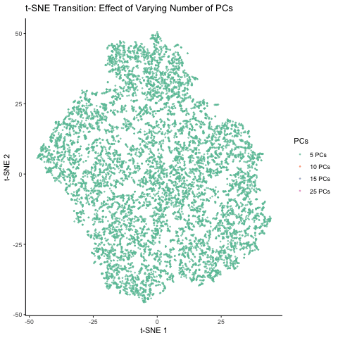
This figure visualizes the effect of varying the number of principal components (PCs) used in t-SNE for dimensionality reduction on a spatial transcriptomics dataset. The animation transitions smoothly between t-SNE visualizations based on different numbers of PCs: 5, 10, 15, and 25. Each t-SNE plot represents the clustering and distribution of the dataset in a reduced 2D space, with points colored according to the number of PCs used in the analysis. By examining the animation, we can observe how increasing the number of PCs affects the spatial organization and separability of the data, highlighting the impact of dimensionality reduction on capturing variance and patterns within the dataset.

library(ggplot2)
library(Rtsne)
library(gganimate)
library(dplyr)
library(patchwork)
library(RColorBrewer)
library(tidyr)

# Load dataset
data <- read.csv('~/Desktop/genomic-data-visualization-2025/data/codex_spleen_3.csv.gz', row.names = 1)

# Extract relevant data
position <- data[, 1:2]
gexp <- data[, 4:31]  

# Normalize gene expression
norm_expr <- log1p(gexp / rowSums(gexp) * mean(rowSums(gexp)) + 1)

# Perform PCA
top_pcs <- prcomp(norm_expr, center = TRUE, scale. = TRUE)
num_pcs <- min(ncol(top_pcs$x), 25) 

# Run t-SNE on varying numbers of PCs
set.seed(42)
tsne_5pcs <- Rtsne(top_pcs$x[, 1:5], perplexity = 30, max_iter = 1000)$Y
set.seed(42)
tsne_10pcs <- Rtsne(top_pcs$x[, 1:10], perplexity = 30, max_iter = 1000)$Y
set.seed(42)
tsne_15pcs <- Rtsne(top_pcs$x[, 1:15], perplexity = 30, max_iter = 1000)$Y
if (num_pcs >= 25) {
  set.seed(42)
  tsne_25pcs <- Rtsne(top_pcs$x[, 1:25], perplexity = 30, max_iter = 1000)$Y
} else {
  tsne_25pcs <- NULL
}

# Create a smoothly transitioning dataset with correct PC order
tsne_df <- data.frame(
  ID = rep(1:nrow(tsne_5pcs), if (is.null(tsne_25pcs)) 3 else 4),
  X1 = c(tsne_5pcs[,1], tsne_10pcs[,1], tsne_15pcs[,1], if (!is.null(tsne_25pcs)) tsne_25pcs[,1] else NULL),
  X2 = c(tsne_5pcs[,2], tsne_10pcs[,2], tsne_15pcs[,2], if (!is.null(tsne_25pcs)) tsne_25pcs[,2] else NULL),
  PCs = rep(c("5 PCs", "10 PCs", "15 PCs", if (!is.null(tsne_25pcs)) "25 PCs" else NULL), each = nrow(tsne_5pcs))
)

# Reorder factor levels to ensure the correct animation order
tsne_df$PCs <- factor(tsne_df$PCs, levels = c("5 PCs", "10 PCs", "15 PCs", "25 PCs"))

# Define color palette
palette <- brewer.pal(if (is.null(tsne_25pcs)) 3 else 4, "Set2")

# Create smoothly transitioning animation
p <- ggplot(tsne_df, aes(X1, X2, group = ID, color = PCs)) +
  geom_point(alpha = 0.6, size = 0.5) +
  scale_color_manual(values = palette) +
  theme_classic() +
  labs(title = "t-SNE Transition: Effect of Varying Number of PCs", x = "t-SNE 1", y = "t-SNE 2") +
  transition_states(PCs, transition_length = 4, state_length = 2, wrap = FALSE) +
  ease_aes('quadratic-in-out')

# Save animation
animate(p, renderer = gifski_renderer("htauchi1.gif"))