Validating Efficacy of Spatial Capture Spot Transcriptomic Deconvolution in Interrogating Cell Type

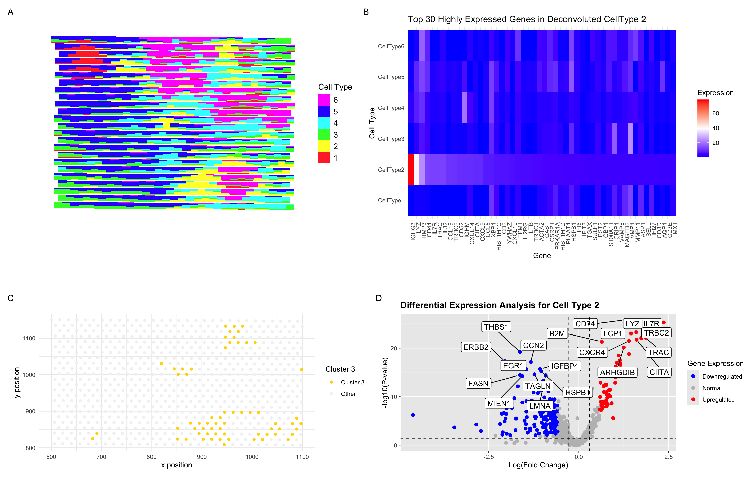
In the previous analysis (HW3), I depicted a visium dataset in embedded space and clustered to identify a B-cell-related cell type. Here, I perform STdeconvolution to parse the cell type composition of each spatial spot, then identify a parsed cell type that is spatially correlated with the B-cell type (cluster 3) from HW3. I identify the cell type 2 (A) as being spatially autocorrelated with the cluster 3 based on spot-based clustering. Analysis of the gene profile of this cell type relative to the other cell types revelas IGHG3 and LYZ as especially potent differentially upregulated genes. IGHG3 is indicative of B-lymphocytes/memory B cells, while LYZ is more suited to myeloid character. The top hits coincide, however, and it is possible that for this cursory gene expression top hit organization (B), LTZ is not necessary most potently upregulated. For the sake of 6-way cell type comparison, however, this heat map is an effective visualization.
In subplot C, I ilustrate the spatial organization of cluster 3 from raw capture spot gene expression data (C), which is highly correlated with the distribution of cell type 2 prevalence in subplot A. In subplot D, I illustrate the differentially expressed genes for celltype 2, which is in line, with potent IL7R and LYZ expression, which coincides with the B cell hypothesis. IL7R is a common surface marker for B cells and T cells. I thus identify a comparable cell type and validate the efficacy of deconvolution methods for spot-based spatial cell type analysis.
1.https://www.ncbi.nlm.nih.gov/gene/4050#:~:text=Lymphotoxin%20beta%20is%20a%20type,Long%20Non%2DCoding%20RNA%20AL928768.
- https://www.uniprot.org/uniprotkb/Q06643/entry
- https://www.proteinatlas.org/ENSG00000227507-LTB
- https://www.proteinatlas.org/ENSG00000090382-LYZ/single+cell
5. Code (paste your code in between the ``` symbols)
1
2
3
4
5
6
7
8
9
10
11
12
13
14
15
16
17
18
19
20
21
22
23
24
25
26
27
28
29
30
31
32
33
34
35
36
37
38
39
40
41
42
43
44
45
46
47
48
49
50
51
52
53
54
55
56
57
58
59
60
61
62
63
64
65
66
67
68
69
70
71
72
73
74
75
76
77
78
79
80
81
82
83
84
85
86
87
88
89
90
91
92
93
94
95
96
97
98
99
100
101
102
103
104
105
106
107
108
109
110
111
112
113
114
115
116
117
118
119
120
121
122
123
124
125
126
127
128
129
130
131
132
133
134
135
136
137
138
139
140
141
142
143
144
145
146
147
148
149
150
151
152
153
154
155
156
157
158
159
160
161
162
163
164
165
166
167
168
169
170
171
172
173
174
175
176
177
178
179
180
181
182
183
184
185
186
187
188
189
190
191
192
193
194
195
196
197
198
199

## GDV EC2
## SV Kammula

#require(remotes)
#remotes::install_github('JEFworks-Lab/STdeconvolve')
library(ggplot2)
library(scatterbar)
library(STdeconvolve)
library(patchwork)
library(dplyr)
library(ggrepel)

data <- read.csv('eevee.csv.gz')

head(data)
pos <- data[,3:4]
colnames(pos) <- c('x', 'y')
cd <- data[, 5:ncol(data)]
rownames(pos) <- rownames(cd) <- data$barcode

counts <- cleanCounts(t(cd), min.lib.size = 100)
## feature select for genes
corpus <- restrictCorpus(counts, removeAbove=1.0, removeBelow = 0.05)
## choose optimal number of cell-types
#ldas <- fitLDA(t(as.matrix(corpus)), Ks = c(8))
ldas <- fitLDA(t(as.matrix(corpus)), Ks = seq(5,10))
## get best model results
optLDA <- optimalModel(models = ldas, opt = "6")
## extract deconvolved cell-type proportions (theta) and transcriptional profiles (beta)
results <- getBetaTheta(optLDA, perc.filt = 0.05, betaScale = 1000)
deconProp <- results$theta
deconGexp <- results$beta
## visualize deconvolved cell-type proportions
vizAllTopics(deconProp, pos,
             r=8, lwd=0)


g1 <- scatterbar(
  deconProp,
  pos,
  size_x = NULL,
  size_y = NULL,
  padding_x = 0,
  padding_y = 0,
  show_legend = TRUE,
  legend_title = "Cell Type",
  colors = NULL,
  verbose = TRUE
  #xlab("x position"),
  #ylab("y position")
)


## heat map expressing cell type 2 gene expression heat map versus other cluster gene expression
## average per cluster 2 and other clusters then ranked heat map


library(ggplot2)
library(dplyr)
library(reshape2)


rownames(deconGexp) <- paste0("CellType", 1:6)
expression_matrix = deconGexp
# unclear gene expression markers, remove for clarity
expression_matrix <- expression_matrix[, !(colnames(expression_matrix) %in% c("JCHAIN", "IGHA1"))]


# Extract the top 30 highest expressed genes in CellType2
top_genes <- expression_matrix["CellType2", ] %>%
  sort(decreasing = TRUE) %>%  # Sort genes by highest expression
  head(50) %>%
  names()  # Get the gene names

# Filter original matrix to keep only these top genes
filtered_matrix <- expression_matrix[, top_genes]

# Convert matrix to long format for ggplot
df_long <- as.data.frame(filtered_matrix) %>%
  mutate(CellType = rownames(expression_matrix)) %>%  # Keep cell type info
  reshape2::melt(id.vars = "CellType", variable.name = "Gene", value.name = "Expression")

# Plot heatmap
g2 <- ggplot(df_long, aes(x = Gene, y = CellType, fill = Expression)) +
  geom_tile() +
  scale_fill_gradientn(colors = c("blue", "white", "red")) +  # Low = blue, high = red
  theme_minimal() +
  labs(title = "Top 30 Highly Expressed Genes in Deconvoluted CellType 2", x = "Gene", y = "Cell Type") +
  theme(axis.text.x = element_text(angle = 90, hjust = 1))  # Rotate x-axis labels for readability


## k means clustering and visualize


gexp <- data[, 5:ncol(data)]

loggexp <- log10(gexp + 1)
com <- kmeans(loggexp, centers = 6)
clusters <- com$cluster
clusters <- as.factor(clusters)
names(clusters) <- rownames (gexp)
head(clusters)

norm <- gexp/rowSums(gexp) * 10000
rowSums(norm)
topgenes <- names(sort(colSums(norm), decreasing=TRUE)[1:1000])
normsub <- norm[,topgenes]

pcs <- prcomp(loggexp)
pos$clusters = clusters
#df <- data.frame(pcs$x, clusters, gene = gexp[, 'CD4'])


emb <- Rtsne::Rtsne(normsub)
df <- data.frame(emb$Y, clusters)
pos$cluster_3 <- ifelse(df$clusters == 3, "Cluster 3", "Other")
g3 <- ggplot(pos, aes(x = x, y = y, col = cluster_3)) +
  geom_point() +
  scale_color_manual(values = c("Cluster 3" = "#FFD700", "Other" = "#F2F2F2")) +
  labs(color = "Cluster 3") +
  #scale_size(range = c(0.5, 1.0)) +
  theme_minimal() +
  #ggtitle('Spleen Spatial Panel with Cluster 3 Colored') +
  xlab("x position") +
  ylab("y position") +
  guides(size = "none")
  #theme(legend.position = "none")


### volcano of differential expression in cell type 2

# Differential expression analysis for clustering cluster 2
pv_2 <- sapply(colnames(normsub), function(i) {
  wilcox.test(normsub[clusters == "3", i], normsub[clusters != "3", i])$p.value
})
logfc_2 <- sapply(colnames(normsub), function(i) {
  log2(mean(normsub[clusters == "3", i]) / mean(normsub[clusters != "3", i]))
})

df_diffexp_2 <- data.frame(gene = colnames(normsub), logfc_2, logpv_2 = -log10(pv_2 + 1e-300))
df_diffexp_2$diffexp <- "Not Significant"
df_diffexp_2[df_diffexp_2$logpv_2 > 2 & df_diffexp_2$logfc_2 > 0.58, "diffexp"] <- "Upregulated"
df_diffexp_2[df_diffexp_2$logpv_2 > 2 & df_diffexp_2$logfc_2 < -0.58, "diffexp"] <- "Downregulated"

df_diffexp_2$diffexp <- as.factor(df_diffexp_2$diffexp)

upregulated_genes_2 <- df_diffexp_2 %>%
  filter(diffexp == "Upregulated") %>%
  arrange(desc(logpv_2)) %>%
  head(10)

downregulated_genes_2 <- df_diffexp_2 %>%
  filter(diffexp == "Downregulated") %>%
  arrange(desc(logpv_2)) %>%
  head(10)

labeled_genes_2 <- bind_rows(upregulated_genes_2, downregulated_genes_2)

g4 <- ggplot(df_diffexp_2, aes(x = logfc_2, y = logpv_2, col = diffexp)) +
  geom_point(size = 2) +
  geom_label_repel(data = labeled_genes_2, aes(label = gene), box.padding = 0.5,  point.padding = 0.5,
                   segment.color = 'black', fill = "white", color = "black", max.overlaps = 25,
                   force = 4, size = 4) +
  ylim(0, max(df_diffexp_2$logpv_2, na.rm = TRUE) + 5) +
  geom_hline(yintercept = -log10(0.05), linetype = "dashed") +
  geom_vline(xintercept = c(-0.3, 0.3), linetype = "dashed") +
  labs(col = "Gene Expression",
       title = "Differential Expression Analysis for Cell Type 2",
       x = "Log(Fold Change)",
       y = "-log10(P-value)") +
  scale_y_continuous() +
  scale_x_continuous() +
  scale_color_manual(values = c("blue", "grey", "red"), labels = c("Downregulated", "Normal", "Upregulated")) +
  theme(plot.title = element_text(face = "bold"),
        aspect.ratio = 0.5)

##


(g1 + g2) / (g3 + g4) + plot_annotation(tag_levels = 'A')


###