HW2: Spatial gene expression with PCA

1. What data types are you visualizing?
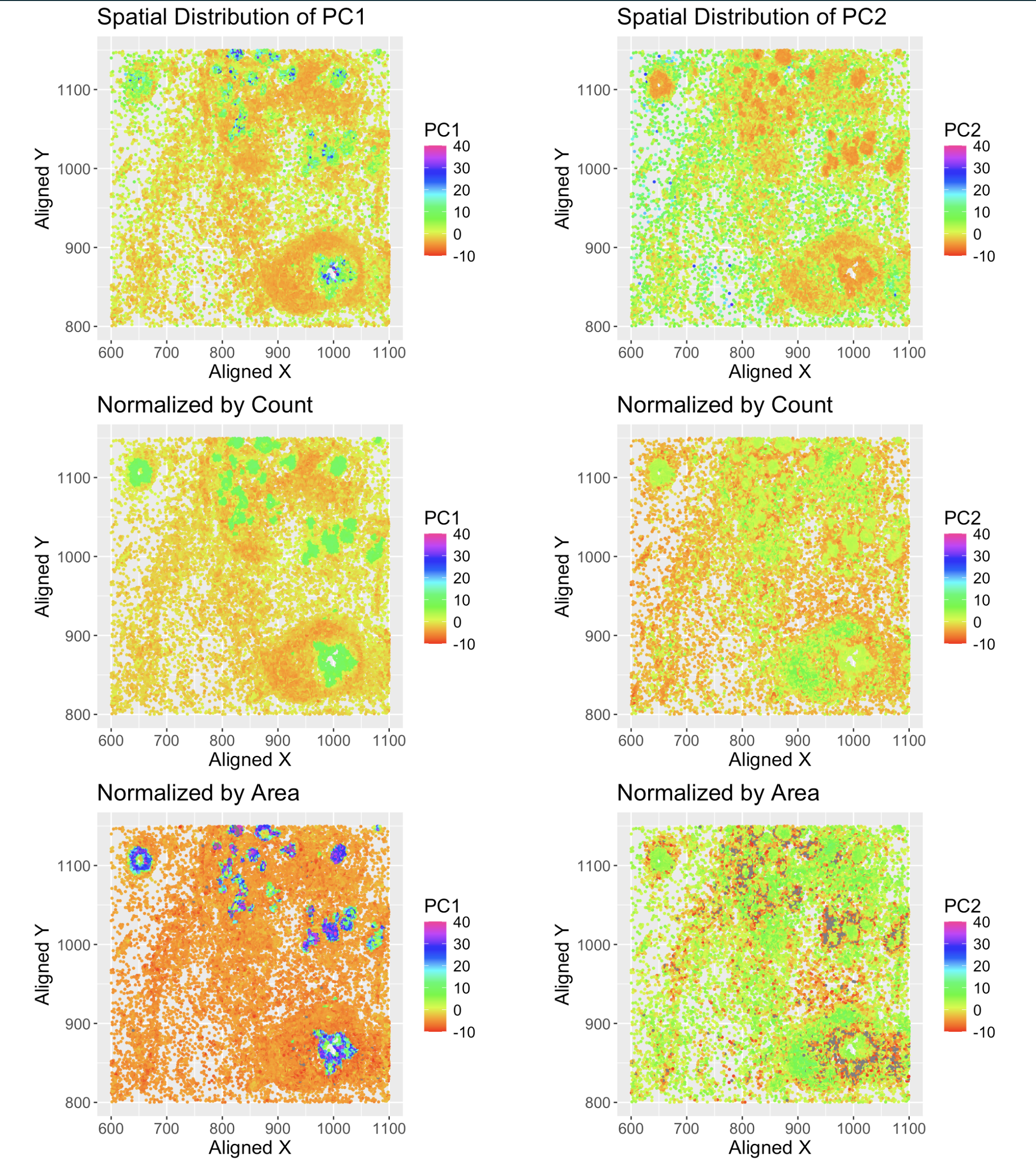
- Spatial data of each cell, the x, y coordinates of the cell location.
- Quantitative: each dot is color coded with the 1st principal component, PC1 as well as PC2. The color is mapped to the value of the PC1 and PC2.
- Same process was repeated using normalized data, shown in the bottom row. Each row is normalized by the total count of all genes in each cell as a proxy to account for the cell size and densiy.
2. What data encodings (geometric primitives and visual channels) are you using to visualize these data types?
- Used the points as geometric primitive for each cell positioned by x and y coordinates.
- Used color to encode the values of PC1 and PC2 respectively. Note that their ranges are set to the same range to make the color mapping consistent across all plots for better comparison.
3. What about the data are you trying to make salient through this data visualization?
The intention is to use the PCA to reduce the dimensionality of the data and visualize the relationship between overall gene expression level vs spatial distribution of the cells. PCA allows us to have the compact representation of the data and visualize the values in reduced space.
Also, by using different normalization methods, we can see how the spatial distribution of the cells changes when we account for the cell size and density and how they affect the gene expression levels.
Also, by using different normalization methods, we can see how the spatial distribution of the cells changes when we account for the cell size and density and how they affect the gene expression levels.
4. What Gestalt principles or knowledge about perceptiveness of visual encodings are you using to accomplish this?
- Similarity: cells with similar values of PC1 and PC2 are represented by similar colors.
- Proximity of the dots to each other shows the spatial distribution of the gene across the cells.
- As the plot shows indeed the cells with similar gene expression levels are located close to each other and follow the spatial distribution of the cells.
5. Code (paste your code in between the ``` symbols)
1
2
3
4
5
6
7
8
9
10
11
12
13
14
15
16
17
18
19
20
21
22
23
24
25
26
27
28
29
30
31
32
file <- 'pikachu.csv.gz' # please chage the file name to your data file
data <- read.csv(file, row.names=1)

library(gridExtra)
library(ggplot2)
library(stats)

gexp <- data[, 7:ncol(data)]
normed_gexp <- gexp/rowSums(gexp)
area_normed_gexp <- gexp/data$cell_area*10

# PCA
pca <- prcomp(gexp, scale=TRUE)
normed_pca <- prcomp(normed_gexp, scale=TRUE)
area_normed_pca <- prcomp(area_normed_gexp)

df <- data.frame(pca$x)
normed_df <- data.frame(normed_pca$x)
data_pca <- cbind(data, pca$x)
data_normed_pca <- cbind(data, normed_df)
data_area_normed_pca <- cbind(data, area_normed_pca$x)

grid.arrange(
  ggplot(data_pca) + geom_point(aes(x=aligned_x, y=aligned_y, color=PC1), size=0.5) + ggtitle("Spatial Distribution of PC1") + theme(aspect.ratio=1.0) + scale_color_gradientn(colors = rainbow(10), limits=c(-10, 40)) + xlab("Aligned X") + ylab("Aligned Y") + theme(text = element_text(size=15)),
  ggplot(data_pca) + geom_point(aes(x=aligned_x, y=aligned_y, color=PC2), size=0.5) + ggtitle("Spatial Distribution of PC2") + theme(aspect.ratio=1.0) + scale_color_gradientn(colors = rainbow(10), limits=c(-10, 40)) + xlab("Aligned X") + ylab("Aligned Y") + theme(text = element_text(size=15)),
  ggplot(data_normed_pca) + geom_point(aes(x=aligned_x, y=aligned_y, color=PC1), size=0.5) + ggtitle("Normalized by Count") + theme(aspect.ratio=1.0) + scale_color_gradientn(colors = rainbow(10), limits=c(-10, 40)) + xlab("Aligned X") + ylab("Aligned Y") + theme(text = element_text(size=15)),
  ggplot(data_normed_pca) + geom_point(aes(x=aligned_x, y=aligned_y, color=PC2), size=0.5) + ggtitle("Normalized by Count") + theme(aspect.ratio=1.0) + scale_color_gradientn(colors = rainbow(10), limits=c(-10, 40)) + xlab("Aligned X") + ylab("Aligned Y") + theme(text = element_text(size=15)),
  ggplot(data_area_normed_pca) + geom_point(aes(x=aligned_x, y=aligned_y, color=PC1), size=0.5) + ggtitle("Normalized by Area") + theme(aspect.ratio=1.0) + scale_color_gradientn(colors = rainbow(10), limits=c(-10, 40)) + xlab("Aligned X") + ylab("Aligned Y") + theme(text = element_text(size=15)),
  ggplot(data_area_normed_pca) + geom_point(aes(x=aligned_x, y=aligned_y, color=PC2), size=0.5) + ggtitle("Normalized by Area") + theme(aspect.ratio=1.0) + scale_color_gradientn(colors = rainbow(10), limits=c(-10, 40)) + xlab("Aligned X") + ylab("Aligned Y") + theme(text = element_text(size=15)),
  ncol = 2
)