Impact of Gene Expression Mean and Variance on PCA Loadings: Scaled vs. Unscaled Data

1. What data types are you visualizing?
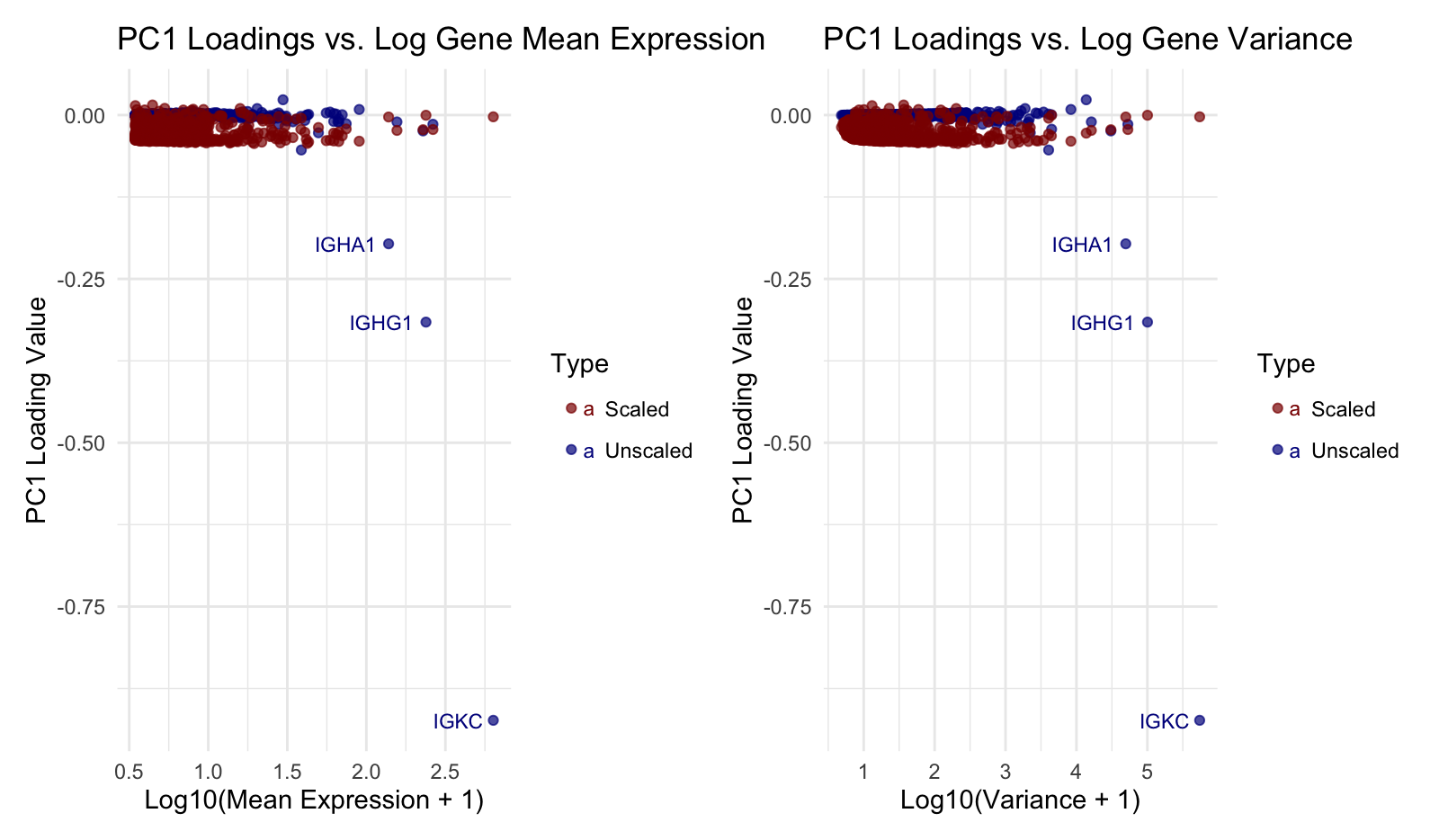
I am visualizing quantitative data for gene expression statistics. Specifically, I compare gene mean expression and variance (log-transformed) against PC1 loading values from PCA. Additionally, I’m visualizing categorical data (scaled vs. unscaled PCA), distinguishing them by color.
2. What data encodings (geometric primitives and visual channels) are you using to visualize these data types?
I am using the geometric primitive of points to represent each cell. Position on the x-axis encodes log-transformed gene expression mean (left) and variance (right), while position on the y-axis encodes PC1 loading values. Hue (red for scaled, blue for unscaled) differentiates PCA approaches. Text labels highlight outlier genes with extreme PC1 loadings. I also use saturation to declutter points.
3. What about the data are you trying to make salient through this data visualization?
This visualization highlights the relationship between gene expression properties (mean and variance) and their influence on the first principal component (PC1) in PCA. Specifically, it examines whether highly expressed or highly variable genes contribute more to PC1 and how this relationship changes when the data is scaled. By distinguishing between scaled and unscaled PCA, it makes salient how PCA behaves differently when expression values are standardized. Additionally, outlier genes with extreme PC1 loadings are labeled, drawing attention to genes that disproportionately drive transcriptional variation.
4. What Gestalt principles or knowledge about perceptiveness of visual encodings are you using to accomplish this?
Similarity is used by using color (red for scaled, blue for unscaled) to group data points based on their transformation method, making it easy to compare the effects of scaling. Proximity is used to group data points with similar PC1 loading values, reinforcing the clustering of most genes near zero while highlighting outliers.
5. Code (paste your code in between the ``` symbols)
1
2
3
4
5
6
7
8
9
10
11
12
13
14
15
16
17
18
19
20
21
22
23
24
25
26
27
28
29
30
31
32
33
34
35
36
37
38
39
40
41
42
43
44
45
46
47
48
49
50
51
52
53
54
55
56
57
58
59
60
61
62
63
64
65
66
67
68
69
70
71
72
library(ggplot2)
library(patchwork)

# Load dataset
file <- 'eevee.csv.gz'
data <- read.csv(file)

# Extract gene expression matrix
gexp <- data[, 7:ncol(data)]
rownames(gexp) <- data$barcode

# Select top 1000 highly expressed genes
topgenes <- names(sort(colSums(gexp), decreasing = TRUE)[1:1000])
gexpsub <- gexp[, topgenes]

# Compute mean and variance of each gene
gene_means <- colMeans(gexpsub)
gene_vars <- apply(gexpsub, 2, var)

# Perform PCA without scaling
pcs_unscaled <- prcomp(gexpsub, scale = FALSE)
pc1_loadings_unscaled <- pcs_unscaled$rotation[, 1]

# Perform PCA with scaling
pcs_scaled <- prcomp(gexpsub, scale = TRUE)
pc1_loadings_scaled <- pcs_scaled$rotation[, 1]

# Create data frames for plotting (apply log transformation to mean & variance)
df_unscaled <- data.frame(
  mean = log10(gene_means + 1),
  variance = log10(gene_vars + 1),
  loading = pc1_loadings_unscaled,
  Type = "Unscaled",
  Gene = names(gene_means)
)

df_scaled <- data.frame(
  mean = log10(gene_means + 1),
  variance = log10(gene_vars + 1),
  loading = pc1_loadings_scaled,
  Type = "Scaled",
  Gene = names(gene_means)
)

df_combined <- rbind(df_unscaled, df_scaled)

# Filter for genes with PC1 loading less than -0.1
df_combined$label <- ifelse(df_combined$loading < -0.1, df_combined$Gene, NA)

# Panel 1: PC1 Loadings vs. Log-Transformed Gene Mean Expression
p1 <- ggplot(df_combined, aes(x = mean, y = loading, color = Type)) +
  geom_point(alpha = 0.7) +
  geom_text(aes(label = label), na.rm = TRUE, size = 3, hjust = 1.2, vjust = 0.5) +  # Move label left
  scale_color_manual(values = c("darkred", "darkblue")) +
  theme_minimal() +
  labs(title = "PC1 Loadings vs. Log Gene Mean Expression",
       x = "Log10(Mean Expression + 1)", y = "PC1 Loading Value")

# Panel 2: PC1 Loadings vs. Log-Transformed Gene Variance
p2 <- ggplot(df_combined, aes(x = variance, y = loading, color = Type)) +
  geom_point(alpha = 0.7) +
  geom_text(aes(label = label), na.rm = TRUE, size = 3, hjust = 1.2, vjust = 0.5) +  # Move label left
  scale_color_manual(values = c("darkred", "darkblue")) +
  theme_minimal() +
  labs(title = "PC1 Loadings vs. Log Gene Variance",
       x = "Log10(Variance + 1)", y = "PC1 Loading Value")

# Combine plots using patchwork
final_plot <- p1 | p2
print(final_plot)

## ChatGPT used to help comment code and add labels to certain points.