Comparison of Scaled and Unscaled PCA: Gene Mean Expression, Variance, and PC1 Loadings

1. What data types are you visualizing?
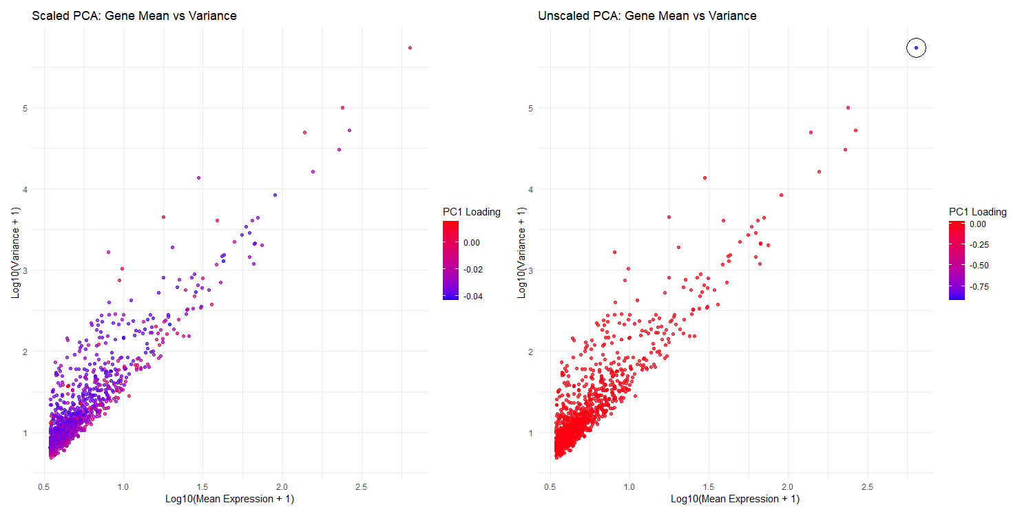
I am visualizing quantitative data, which includes log-transformed mean expression (x-axis), log-transformed variance (y-axis), and PC1 loading values (color hue).
2. What data encodings (geometric primitives and visual channels) are you using to visualize these data types?
Geometric primitives: I am using points in two plots to represent genes.
Visual channels: Mean expression of genes are encoded as the position on the x-axis (in both plots). Variance of expression for each gene is encoded as the position on the y-axis.
Color (hue) is used to encode PC1 loading values (represented as a gradient from red to blue).
3. What about the data are you trying to make salient through this data visualization?
I am trying to answer question 2, which focuses on gene loadings and PCs. Specifically, these 2 plots compare and contrast between scaled and unscaled PCA, and explore the effect of scaling on PC1 loading values. It could be observed that without scaling in PCA, genes with higher variance dominate PC1 loading values (circled outlier as shown), while if PCA is scaled (all genes weighted equally), there is a balanced contribution from genes and no dominance from high-variance genes.
4. What Gestalt principles or knowledge about perceptiveness of visual encodings are you using to accomplish this?
I am using Gestalt principles of similarity, proximity, and enclosure in my 2 plots.
Similarity: points of similar color (hue) will be perceived as the same group, as they will have similar PC1 loading values.
Proximity: points close to each other will be perceived as a related group, as they have similar values of mean and variance of expression.
Enclosure: (in the unscaled PCA plot only) I enclosed the outlier with a circle, highlighting its difference from other data points (high mean/variance, and high PC1 loading values).
5. Code (paste your code in between the ``` symbols)
1
2
3
4
5
6
7
8
9
10
11
12
13
14
15
16
17
18
19
20
21
22
23
24
25
26
27
28
29
30
31
32
33
34
35
36
37
38
39
40
41
42
43
44
45
46
47
48
49
50
51
52
53
54
55
56
57
58
59
60
61
62
63
64
65
66
67
68
## PRE-PROCESSING
library(ggplot2)
library(patchwork)
file <- 'D:/Spring 2025/GDV/genomic-data-visualization-2025/data/eevee.csv.gz'
data <- read.csv(file)

# Extract gene expression data
gexp <- data[, 5:ncol(data)]
rownames(gexp) <- data$barcode

# Limit to top 1000 most highly expressed genes
topgenes <- names(sort(colSums(gexp), decreasing = TRUE)[1:1000])
gexpsub <- gexp[, topgenes]

## PCA
# Perform PCA with and without scaling
pcs_scaled <- prcomp(gexpsub, scale. = TRUE)
pcs_unscaled <- prcomp(gexpsub, scale. = FALSE)

# Create dfs for scaled and unscaled PCA
# include loading values on the 1st PC, mean expression, and variance of expression of each gene
scaled_df <- data.frame(
  PC1_loading = pcs_scaled$rotation[, 1],
  Mean = colMeans(gexpsub),
  Variance = apply(gexpsub, 2, var)
)

unscaled_df <- data.frame(
  PC1_loading = pcs_unscaled$rotation[, 1],
  Mean = colMeans(gexpsub),
  Variance = apply(gexpsub, 2, var)
)

# Log-transform the data
scaled_df$Mean_log <- log10(scaled_df$Mean + 1)
scaled_df$Variance_log <- log10(scaled_df$Variance + 1)
unscaled_df$Mean_log <- log10(unscaled_df$Mean + 1)
unscaled_df$Variance_log <- log10(unscaled_df$Variance + 1)

# Identify the outlier in the unscaled PCA plot for further processing
outlier <- unscaled_df[which.max(unscaled_df$Variance_log), ]

## PLOTTING
# Scaled PCA
plot_scaled <- ggplot(scaled_df, aes(x = Mean_log, y = Variance_log, color = PC1_loading)) +
  geom_point(alpha = 0.7) +
  scale_color_gradient(low = "blue", high = "red") +
  labs(title = "Scaled PCA: Gene Mean vs Variance", x = "Log10(Mean Expression + 1)", y = "Log10(Variance + 1)", color = "PC1 Loading") +
  theme_minimal()

# Unscaled PCA with outlier circled
plot_unscaled <- ggplot(unscaled_df, aes(x = Mean_log, y = Variance_log, color = PC1_loading)) +
  geom_point(alpha = 0.7) +
  geom_point(data = outlier, aes(x = Mean_log, y = Variance_log), shape = 1, size = 10, color = "black") +
  scale_color_gradient(low = "blue", high = "red") +
  labs(title = "Unscaled PCA: Gene Mean vs Variance", x = "Log10(Mean Expression + 1)", y = "Log10(Variance + 1)", color = "PC1 Loading") +
  theme_minimal()

# Plot using patchwork
plot_scaled + plot_unscaled

# References
# Prof Fan's class code for pre-processing eevee data
# https://www.rdocumentation.org/packages/stats/versions/3.6.2/topics/prcomp
# https://rstudio.github.io/cheatsheets/data-visualization.pdf
# https://www.geeksforgeeks.org/return-the-index-of-the-first-maximum-value-of-a-numeric-vector-in-r-programming-which-max-function/
# https://ggplot2.tidyverse.org/reference/scale_gradient.html
# https://www.rdocumentation.org/packages/base/versions/3.6.2/topics/data.frame