Spatial Transcriptomics Reveals a Distinct Epithelial Cell Population Defined by ELF3 Expression: A Multi-Dimensional Analysis of the Cluster in Interest

1. Describe your figure briefly so we know what you are depicting. Write a description to convince me that your cluster interpretation is correct.
Figure Description and Interpretation
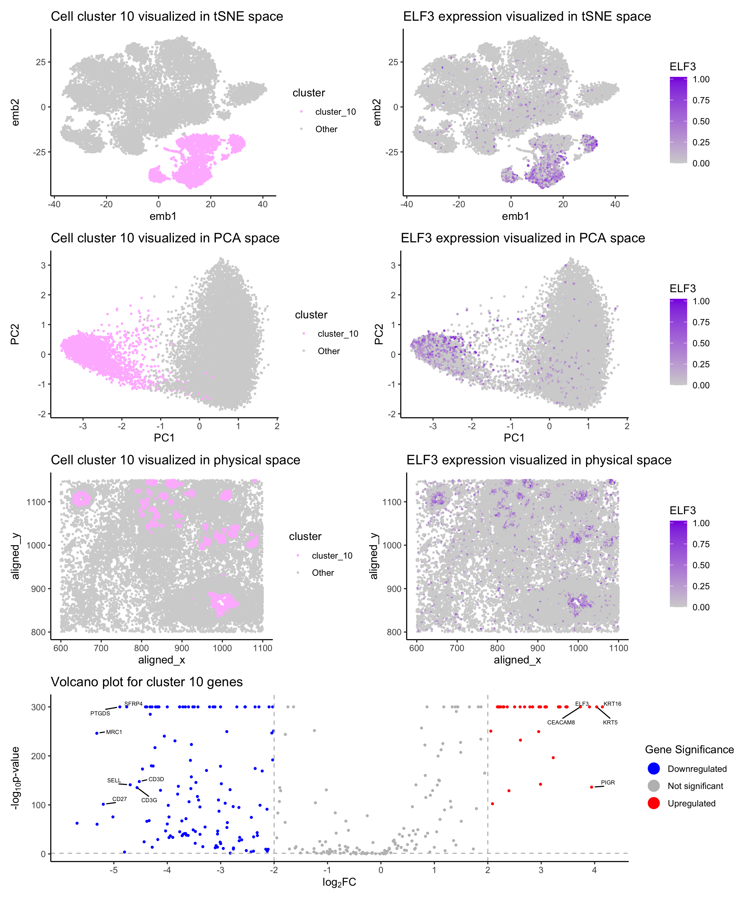
This figure presents a multi-dimensional analysis of Cluster 10, a cell group identified via k-means clustering (k = 10) of single-cell gene expression data. The panels are organized into four rows that together demonstrate both the distinct spatial distribution and unique gene expression profile of Cluster 10.
tSNE Space (Row 1) Plot A: A tSNE map displays Cluster 10 highlighted in plum pink against a gray background representing other clusters. The clear separation of Cluster 10 in this nonlinear projection suggests that these cells form a unique population. Plot B: Overlaying the expression of ELF3 (a key transcription factor) on the tSNE space using a gradient from gray (low) to blueviolet (high) reveals that cells in Cluster 10 express ELF3 at significantly higher levels compared to surrounding clusters.
PCA Space (Row 2) Plot C: A PCA plot similarly emphasizes the segregation of Cluster 10 in a linear dimensionality reduction framework, corroborating the distinctiveness observed in the tSNE analysis. Plot D: Mapping ELF3 expression onto the PCA space reinforces that high ELF3 expression aligns with the cells in Cluster 10, supporting the marker’s role in defining this cluster.
Physical Tissue Space (Row 3) Plot E: The spatial visualization of cells on the tissue section shows that Cluster 10 occupies a defined region, suggesting that these cells are not only transcriptionally distinct but also localized within specific tissue microenvironments. Plot F: The spatial distribution of ELF3 expression mirrors that of Cluster 10, further indicating that ELF3 is a hallmark of the cells’ identity in this cluster.
Differential Expression (Volcano Plot, Row 4) Plot G: A volcano plot displays differentially expressed genes in Cluster 10 compared to all other clusters. The gene ELF3 is highlighted as a significantly upregulated gene in Cluster 10, along with KRT16 and KRT5. Downregulated genes such as PTGDS and MRC1 are also labeled. Based on the volcano plot, ELF3 was chosen as a marker gene for Cluster 10 due to its significant upregulation and potential biological relevance. The expression of ELF3 is further visualized in tSNE, PCA, and physical space to confirm its association with Cluster 10.
Supporting Evidence and Biological Context
The high expression of ELF3 in Cluster 10 is significant for our interpretation. ELF3 (E74-like factor 3) is an epithelial-specific transcription factor known to regulate genes involved in epithelial differentiation, cell adhesion, and maintenance of tissue architecture. Its role in promoting epithelial cell identity has been well documented. For instance: Otero et al. (2009) demonstrated that ELF3 is crucial for maintaining epithelial differentiation and that its dysregulation can contribute to cancer progression by affecting cell adhesion and migration. Sengez et al. (2019) provided evidence that ELF3 helps suppress the epithelial-mesenchymal transition (EMT), further supporting its role as a guardian of epithelial characteristics. According to The Human Protein Atlas, ELF3 exhibits high RNA expression in respiratory epithelial cells, which aligns with our findings that Cluster 10 represents an epithelial cell population (The Human Protein Atlas, 2023). The co-expression of keratin genes (e.g., KRT16 and KRT5) along with ELF3 in Cluster 10 lends additional support to an epithelial cell identity. Keratins are well-established markers of epithelial cells, and their upregulation is consistent with the transcriptional profile expected from differentiated epithelial populations (Chilosi et al., 2002).
Conclusion: The integration of dimensionality reduction (tSNE and PCA), spatial mapping, and differential expression analyses in the figure robustly indicates that Cluster 10 represents a distinct epithelial cell population. The high expression of ELF3—supported by its documented role in epithelial differentiation and maintenance—along with other epithelial markers, substantiates this interpretation. The association of ELF3 with respiratory epithelial cells, as reported by The Human Protein Atlas, further strengthens the epithelial identity of Cluster 10. To further verify the physical location of Cluster 10, it would be beneficial to explore breast tissue cross-section scans available online, which I currently lack and will need to investigate further.
References: Suzuki, M., et al. “E74-Like Factor 3 Is a Key Regulator of Epithelial Integrity and Immune Response Genes in Biliary Tract Cancer.” Cancer Research, vol. 81, no. 2, 15 Jan. 2021, pp. 489-500. doi:10.1158/0008-5472.CAN-19-2988. Epub 8 Dec. 2020. PMID: 33293429. Subbalakshmi, Ayalur Raghu, et al. “The ELF3 Transcription Factor Is Associated with an Epithelial Phenotype and Represses Epithelial-Mesenchymal Transition.” Journal of Biological Engineering, vol. 17, no. 1, 2 Mar. 2023, p. 17. doi:10.1186/s13036-023-00333-z. Sengez, Burcu, et al. “The Transcription Factor Elf3 Is Essential for a Successful Mesenchymal to Epithelial Transition.” Cells, vol. 8, no. 8, 9 Aug. 2019, p. 858. doi:10.3390/cells8080858. The Human Protein Atlas. “ELF3 - Cell Type RNA Expression, Single Cell Type Expression Cluster: Respiratory Epithelial Cells.” 2023. Available at: https://www.proteinatlas.org.
2. Code (paste your code in between the ``` symbols)
1
2
3
4
5
6
7
8
9
10
11
12
13
14
15
16
17
18
19
20
21
22
23
24
25
26
27
28
29
30
31
32
33
34
35
36
37
38
39
40
41
42
43
44
45
46
47
48
49
50
51
52
53
54
55
56
57
58
59
60
61
62
63
64
65
66
67
68
69
70
71
72
73
74
75
76
77
78
79
80
81
82
83
84
85
86
87
88
89
90
91
92
93
94
95
96
97
98
99
100
101
102
103
104
105
106
107
108
109
110
111
112
113
114
115
116
117
118
119
120
121
122
123
124
125
126
127
128
129
130
131
132
133
134
135
136
137
138
139
140
141
142
143
144
145
146
147
148
149
150
151
152
153
154
155
156
157
158
159
160
161
162
163
164
165
166
167
168
169
170
171
172
173
174
175
176
177
178
179
180
181
182
183
# Load the data
data <- read.csv('~/Desktop/genomic_data_visualization/genomic-data-visualization-2025/data/pikachu.csv.gz')

# Import libraries
library(ggplot2)
library(patchwork)
library(Rtsne)
library(ggrepel)

# Extract physical coordinates and gene expression data
pos <- data[, 5:6]
rownames(pos) <- data$cell_id
gexp <- data[, 7:ncol(data)]
rownames(gexp) <- data$cell_id

# Normalize and log-transform the gene expression data
gexpnorm <- log10(gexp/rowSums(gexp) * mean(rowSums(gexp)) + 1)

# Perform PCA
pcs <- prcomp(gexpnorm)
plot(pcs$sdev[1:30])

# Perform tSNE
tsne <- Rtsne(pcs$x[, 1:20])$Y
ggplot(data.frame(tsne)) + geom_point(aes(x = X1, y = X2), size = 0.05) + theme_classic()

# Check total within-cluster to find optimal k
totw <- sapply(2:25, function(k) {
  com <- kmeans(tsne, centers = k)
  return(com$tot.withinss)
})
plot(2:25, totw, type = "b", pch = 19, col = "purple",
     xlab = "Number of Clusters (k)", ylab = "Total Withiness",
     main = "Total Withinness for Optimal k")

# Perform k-means clustering with chosen k = 10
kmeans_result <- kmeans(tsne, centers = 10)
clusters <- as.factor(kmeans_result$cluster)

# Look at all groups to choose one from
names(clusters) <- rownames(gexpnorm)
df <- data.frame(pcs$x, clusters)
ggplot(df, aes(x=PC1, y=PC2, col=clusters)) + geom_point(size=0.05)

# Define color for the chosen cluster
cluster.cols <- c("plum1", "lightgrey")
names(cluster.cols) <- c("cluster_10", "Other")
selected_cluster <- 10

# Create a new data frame for plotting in tSNE space
df_tsne <- data.frame(
  emb1 = tsne[, 1],
  emb2 = tsne[, 2],
  cluster = ifelse(kmeans_result$cluster == selected_cluster, "cluster_10", "Other")
)

# Plot cluster 10 in tSNE space
p1 <- ggplot(df_tsne, aes(x = emb1, y = emb2, col = cluster)) +
  geom_point(size = 0.5) +
  theme_classic() +
  scale_color_manual(values = cluster.cols) +
  ggtitle("Cell cluster 10 visualized in tSNE space")

# Create a new data frame for plotting in PCA space
df_pca <- data.frame(pcs$x,
                     cluster = ifelse(kmeans_result$cluster == selected_cluster,
                    "cluster_10", "Other"))

# Plot cluster 10 in PCA space
p2 <- ggplot(df_pca, aes(x = PC1, y = PC2, col = cluster)) +
  geom_point(size = 0.5) +
  theme_classic() +
  scale_color_manual(values = cluster.cols) +
  ggtitle("Cell cluster 10 visualized in PCA space")

# Create a new data frame for plotting in physical space
df_phys <- data.frame(
  aligned_x = data$aligned_x,
  aligned_y = data$aligned_y,
  cluster = ifelse(kmeans_result$cluster == selected_cluster, "cluster_10", "Other")
)

# Plot cluster 10 in physical space
p3 <- ggplot(df_phys, aes(x = aligned_x, y = aligned_y, col = cluster)) +
  geom_point(size = 0.5) +
  theme_classic() +
  scale_color_manual(values = cluster.cols) +
  ggtitle("Cell cluster 10 visualized in physical space")

# do wilcox for DE genes
pv <- sapply(colnames(gexpnorm), function(i) {
  wilcox.test(gexpnorm[as.numeric(clusters) == selected_cluster, i],
              gexpnorm[as.numeric(clusters) != selected_cluster, i])$p.value
})

# Avoid p-values of 0
pv[pv == 0] <- 1e-400

# Compute log fold change
logfc <- sapply(colnames(gexpnorm), function(i) {
  log2((mean(gexpnorm[as.numeric(clusters) == selected_cluster, i]) + 1e-6) /
         (mean(gexpnorm[as.numeric(clusters) != selected_cluster, i]) + 1e-6))
})

# Disregard extreme outliers
logfc[logfc < -6] <- NA

# Create a data frame for the volcano plot
df <- data.frame(pv = -log10(pv), logfc = logfc)
df$genes <- rownames(df)

# Add significance label
df$diffexpressed <- "Not Significant"
df$diffexpressed[df$logfc > 2 & pv < 0.05] <- "Upregulated"
df$diffexpressed[df$logfc < -2 & pv < 0.05] <- "Downregulated"

# Cap -log10(p-value) at a max value
max_pv <- 300  # Adjust based on plot aesthetics
df$pv <- pmin(df$pv, max_pv)  # Fix capping logic

# Create volcano plot
p4 <- ggplot(df, aes(x = logfc, y = pv, color = diffexpressed)) +
  geom_point(size = 0.75) +
  geom_vline(xintercept = c(-2, 2), col = "gray", linetype = 'dashed') +
  geom_hline(yintercept = -log10(0.05), col = "gray", linetype = 'dashed') +
  scale_color_manual(values = c("blue", "grey", "red"),
                     labels = c("Downregulated", "Not significant", "Upregulated")) +
  theme_classic() +
  labs(color = 'Gene Significance',
       x = expression("log"[2]*"FC"),
       y = expression("-log"[10]*"p-value"),
       title = "Volcano plot for cluster 10 genes") +
  geom_text_repel(aes(label = ifelse(pv > 100 & (logfc < -4.5 | logfc > 3.5), as.character(genes), "")),
                  max.overlaps = 15,
                  box.padding = 0.5,
                  point.padding = 0.3,
                  min.segment.length = 0,
                  segment.color = "black",
                  force = 5,
                  size = 2, color = "black") +
  scale_x_continuous(breaks = seq(-5, 5, 1)) +
  ylim(0, max_pv + 10) +  # Ensures no cut-off points
  guides(size = "none", color = guide_legend(override.aes = list(size = 5)))

# Plot gene ELF3 in tSNE space
plot.df <- data.frame(emb1 = tsne[,1],
                      emb2 = tsne[,2],
                      ELF3 = gexpnorm$ELF3)

p5 <- ggplot(plot.df, aes(emb1, emb2,col=ELF3)) +
  geom_point(size = 0.4) +
  theme_classic() +
  scale_color_gradient(low='lightgrey', high='blueviolet') +
  ggtitle("ELF3 expression visualized in tSNE space")

# Plot gene ELF3 in PCA space
plot.df <- data.frame(pcs$x,
                      ELF3 = gexpnorm$ELF3)

p6 <- ggplot(plot.df, aes(x = PC1, y = PC2, col = ELF3)) +
  geom_point(size = 0.5) +
  theme_classic() +
  scale_color_gradient(low='lightgrey', high='blueviolet') +
  ggtitle("ELF3 expression visualized in PCA space")

# Plot gene ELF3 in physical space
plot.df <- data.frame(aligned_x = data$aligned_x,
                      aligned_y = data$aligned_y,
                      ELF3 = gexpnorm$ELF3)

p7 <- ggplot(plot.df, aes(aligned_x, aligned_y, col=ELF3)) +
  geom_point(size=0.5) +
  theme_classic() +
  scale_color_gradient(low='lightgrey', high='blueviolet') +
  ggtitle("ELF3 expression visualized in physical space")

# plot using patchwork
(p1 + p5) / (p2 + p6) / (p3 + p7) / p4

## References
# https://ggplot2.tidyverse.org/
# https://stackoverflow.com/questions
# https://ggrepel.slowkow.com/