Homework 3: Differentially Expressed Genes analysis

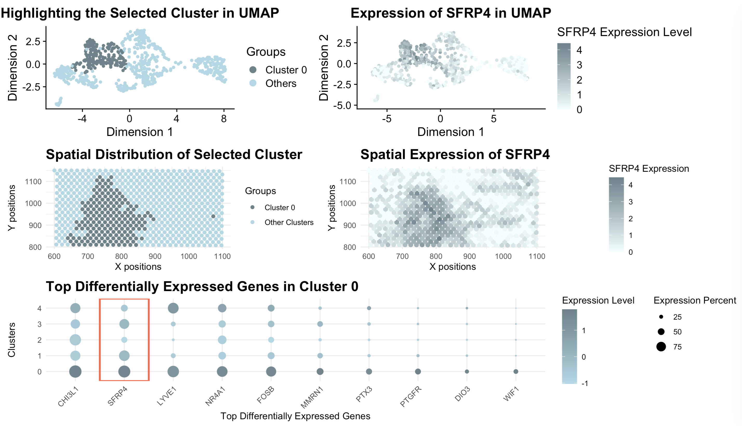
[description] Those panels present a comprehensive visualization of Cluster 0 and its association with the gene SFRP4 through a combination of UMAP, spatial, and gene expression analysis. The top-left UMAP plot highlights Cluster 0 (colored by dark gray) as a distinct group of cells within the low-dimensional space, distinguishing it from other clusters (light blue). SFRP4 is a well-known regulator of the Wnt signaling pathway, often associated with mesenchymal and stromal cell populations in various tissues, particularly in fibrosis, stem cell niches, and cancer microenvironments (Haraguchi et al, 2016). The top-right UMAP plot further illustrates that SFRP4 expression is enriched in similarly specific regions, suggesting its association with Cluster 0. Moving to spatial analysis, the bottom-left panel shows the physical distribution of Cluster 0 cells within the 2D tissue space, revealing a clear localization pattern. Similarly, the bottom-right spatial expression plot confirms that SFRP4 is expressed in the similar region, reinforcing its biological relevance in this cluster. Finally, the bottom dot plot displays the top differentially expressed genes in Cluster 0, where SFRP4 is boxed in red. The dot size represents the percentage of cells expressing each gene, while the color gradient indicates expression intensity. Together, these visualizations demonstrate that Cluster 0 is a distinct, spatially localized population characterized by high SFRP4 expression, suggesting a potential functional role for this gene in the tissue region occupied by this cluster.

Haraguchi, R., Kitazawa, R., Mori, K. et al. sFRP4-dependent Wnt signal modulation is critical for bone remodeling during postnatal development and age-related bone loss. Sci Rep 6, 25198 (2016). https://doi.org/10.1038/srep25198

library(Seurat)
library(ggplot2)
library(patchwork)
library(dplyr)

data = read.csv('./data/eevee.csv.gz')
metadata <- data[, c("barcode", "aligned_x", "aligned_y")]
rownames(metadata) <- metadata$barcode
data <- data[, !colnames(data) %in% c("barcode", "aligned_x", "aligned_y")]
seurat_obj <- CreateSeuratObject(counts = t(data), meta.data = metadata)
seurat_obj <- NormalizeData(seurat_obj)
seurat_obj <- FindVariableFeatures(seurat_obj, selection.method = "vst", nfeatures = 2000)
seurat_obj <- ScaleData(seurat_obj)
seurat_obj <- RunPCA(seurat_obj, features = VariableFeatures(object = seurat_obj))
seurat_obj <- RunUMAP(seurat_obj, dims = 1:30)
seurat_obj <- FindNeighbors(seurat_obj, dims = 1:30)
seurat_obj <- FindClusters(seurat_obj, resolution = 0.5)
# Highlighting one cluster of interest (cluster 0)
seurat_obj$cluster_highlight <- ifelse(Idents(seurat_obj) == "0", "Cluster 0", "Others")
selected_cluster_colors <- c("Cluster 0"="#68838B","Others"="#ADD8E6")
title_theme <- theme(plot.title = element_text(size = 16, face = "bold"))
p1 <- DimPlot(seurat_obj, reduction = "umap", group.by = "cluster_highlight") + 
  ggtitle("Highlighting the Selected Cluster in UMAP") + labs(x = "Dimension 1", y = "Dimension 2") + 
  scale_color_manual(values = selected_cluster_colors,name = "Groups") + title_theme
p2 <- ggplot(metadata, 
             aes(x = aligned_x, 
                 y = aligned_y,
                 color = ifelse(as.factor(Idents(seurat_obj)) == "0", 
                                          "Cluster 0", "Other Clusters"))) +
  geom_point() +
  scale_color_manual(values = c("Cluster 0" = "#68838B", "Other Clusters" = "#ADD8E6"),name = "Groups") +
  theme_minimal() + 
  ggtitle("Spatial Distribution of Selected Cluster") + labs(x = "X positions", y = "Y positions") + title_theme
# Find markers for the selected cluster (cluster 0)
cluster_of_interest <- "0"
markers_cluster <- FindMarkers(seurat_obj, ident.1 = cluster_of_interest, min.pct = 0.25, logfc.threshold = 0.25)
top_gene <- rownames(markers_cluster)[1]  
p3 = FeaturePlot(seurat_obj, features = top_gene) + 
  ggtitle(paste("Expression of", top_gene, "in UMAP")) + labs(x = "Dimension 1", y = "Dimension 2") +
  scale_color_gradientn(colors = c("#F0FFFF","#68838B"), name = "SFRP4 Expression Level") + title_theme
# Create a volcano plot
top_genes <- rownames(markers_cluster[order(markers_cluster$avg_log2FC, decreasing = TRUE),])[1:10]  # Top 10 genes
avg_exp <- AverageExpression(seurat_obj, features = top_genes)$RNA
avg_exp_df <- as.data.frame(avg_exp)
avg_exp_df$gene <- rownames(avg_exp_df)
top_genes_ordered <- avg_exp_df$gene[order(rowMeans(avg_exp_df[,-ncol(avg_exp_df)]), decreasing = TRUE)]
p4 = DotPlot(seurat_obj, features = top_genes_ordered, cols = c("#ADD8E6", "#68838B")) +
  ggtitle("Top Differentially Expressed Genes in Cluster 0") +
  theme_minimal() + labs(x = "Top Differentially Expressed Genes", y = "Clusters") + 
  theme(axis.text.x = element_text(angle = 45, hjust = 1)) + 
  annotate("rect", 
           xmin = which(top_genes_ordered == "SFRP4") - 0.5, 
           xmax = which(top_genes_ordered == "SFRP4") + 0.5, 
           ymin = -Inf, ymax = Inf, 
           color = "#FF6347", fill = NA, size = 1) + title_theme +
  guides(color = guide_colorbar(order = 1, title = "Expression Level"), size = guide_legend(order = 2, title = "Expression Percent")) +  
  theme(
    legend.position = "right",
    legend.box = "horizontal" 
  )
metadata$SFRP4_expression <- FetchData(seurat_obj, vars = "SFRP4")$SFRP4
p5 <- ggplot(metadata, aes(x = aligned_x, y = aligned_y, color = SFRP4_expression)) +
  geom_point(size = 2) +
  scale_color_gradientn(colors = c("#F0FFFF","#68838B"), name = "SFRP4 Expression") +
  theme_minimal() +
  ggtitle("Spatial Expression of SFRP4") +
  labs(x = "X positions", y = "Y positions") + title_theme 

(p1 | p3) / (p2 | p5) / p4