Discovering Epithelial cells

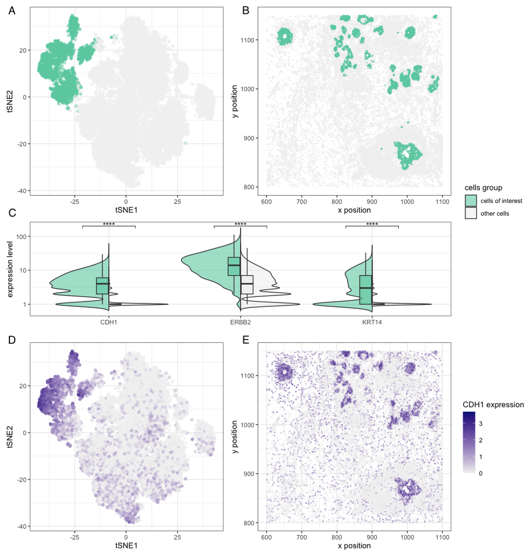
[description] Figures A, B, and C share a common legend and analyze the dataset at the cluster level, where green highlights the cluster of interest and gray represents all other clusters. Figure A presents a tSNE plot applied to log-transformed gene expression data, showing that the cluster of interest is distinctly separated from the rest of the cells. Figure B visualizes the spatial distribution of the cluster of interest and all cells forms a tube-like structure, which supports the clustering results and suggests that these cells may be epithelial. Figure C highlights differential expression of CDH1, ERBB2, and KRT14 between the cluster of interest and other clusters, with these genes selected to further characterize the cluster. CDH1 encodes E-cadherin, a key epithelial marker, while KRT14 and other upregulated keratin genes (not shown in Figure C) encode proteins essential for the epithelial cytoskeleton (1, 2). The elevated expression of ERBB2, along with CDH1 and KRT family genes, suggests that this cluster likely consists of breast cancer cells (2,3,4). Figures D and E analyze CDH1 expression and share a common legend. Figure D displays CDH1 expression on a tSNE plot, where darker blue indicates higher expression, and when compared to Figure A, it is evident that cells with high CDH1 expression form a similar cluster. Figure E maps CDH1 expression in the physical space, showing a pattern consistent with Figure B. Both Figures D and E further validate the clustering results, reinforcing that the cluster of interest is likely epithelial cells.

Reference

1. https://medlineplus.gov/genetics/gene/cdh1/
2. Li, Gang et al. “Keratin gene signature expression drives epithelial-mesenchymal transition through enhanced TGF-β signaling pathway activation and correlates with adverse prognosis in lung adenocarcinoma.” Heliyon vol. 10,3 e24549. 17 Jan. 2024, doi:10.1016/j.heliyon.2024.e24549
3. Xie, Dan et al. “The Potential Role of CDH1 as an Oncogene Combined With Related miRNAs and Their Diagnostic Value in Breast Cancer.” Frontiers in endocrinology vol. 13 916469. 16 Jun. 2022, doi:10.3389/fendo.2022.916469
4. Tan M, Yu D. Molecular Mechanisms of ErbB2-Mediated Breast Cancer Chemoresistance. In: Madame Curie Bioscience Database [Internet]. Austin (TX): Landes Bioscience; 2000-2013. Available from: https://www.ncbi.nlm.nih.gov/books/NBK6194/

library(tidyverse)
library(ggplot2)
library(patchwork)
library(ggpubr) #for stat
library(rstatix) #for stat

pikachu <- read.csv("~/Documents/genom_visual/hw1/pikachu.csv")

exp=log(pikachu[,-c(1:6)]+1)
rownames(exp) <- pikachu$cell_id

set.seed(66)
km=kmeans(exp, centers=6)
clusters <- km$cluster
clusters <- as.factor(clusters) ## tell R it's a categorical variable
names(clusters) <- rownames(exp)

# pcs <- prcomp(exp)
# df <- data.frame(pcs$x, clusters)
# pc=ggplot(df, aes(x=PC1, y=PC2, col=clusters)) + geom_point(alpha=0.5)

emb <- Rtsne::Rtsne(exp)
df <- data.frame(emb$Y)
p1 = ggplot(df, aes(x=X1, y=X2, colour=ifelse(clusters==6, "in","ot"))) + 
  geom_point(alpha=0.5, show.legend = F)+  
  xlab("tSNE1")+
  ylab("tSNE2")+
  scale_color_manual(values = c("in" = "aquamarine3", "ot" = "gray94"))+
  theme_bw()

p2=cbind(pikachu, clusters)%>%
  mutate(clusters=ifelse(clusters==6, "cluster of interest","other clusters"))%>%
  ggplot()+
  geom_point(aes(x = aligned_x, y = aligned_y, colour=clusters), size=0.3, show.legend = F)+
  scale_color_manual(values = c("cluster of interest" = "aquamarine3", "other clusters" = "gray94"))+
  theme_bw()+
  theme(
    panel.grid.major = element_blank(),  # Remove major grid lines
    panel.grid.minor = element_blank()   # Remove minor grid lines
  )+
  xlab("x position")+
  ylab("y position")
  


# c1=exp[names(clusters)[clusters == 6],]
# cr=exp[names(clusters)[clusters != 6],]
# 
# #wilcox.test(c1, cr, alternative = 'greater')
# 
# results <- sapply(1:ncol(exp), function(i) {
#   out <- wilcox.test(c1[,i], cr[,i], alternative = 'greater')
#   out$p.value
# })
# 
# names(results) <- colnames(exp)
# head(sort(results, decreasing = FALSE), n=30) 

comb_stat=pikachu%>%
  select(cell_id,CDH1, KRT14, ERBB2)%>%
  mutate(type=ifelse(cell_id %in% names(clusters)[clusters == 6], "interest", "other")) %>%
  pivot_longer(cols=c("CDH1", "KRT14", "ERBB2"), names_to="gene", values_to="exp")%>%
  group_by(gene)%>%
  wilcox_test(exp~type, alternative = "greater")%>%
  add_significance()%>%
  add_xy_position(x="gene") %>%
  mutate(y.position=2.3)


p3=pikachu%>%
  select(cell_id,CDH1, KRT14, ERBB2)%>%
  mutate(type=ifelse(cell_id %in% names(clusters)[clusters == 6], "cells of interest", "other cells")) %>%
  pivot_longer(cols=c("CDH1", "KRT14", "ERBB2"), names_to="gene", values_to="exp")%>%
  ggplot(aes(x=gene, y=exp+1, fill=type))+
  introdataviz::geom_split_violin(alpha=0.6,trim=FALSE, width=0.9, scale="width")+
  geom_boxplot(width = .2, alpha = .6, outliers = FALSE, show.legend = FALSE)+
  scale_y_log10()+
  stat_pvalue_manual(comb_stat, hide.ns = TRUE, inherit.aes = FALSE)+
  ylab("expression level")+
  xlab("")+
  labs(fill = "cells group")+
  scale_fill_manual(values = c("cells of interest" = "aquamarine3", "other cells" = "gray94"))+
  theme_bw()
  

p4 = ggplot(df, aes(x=X1, y=X2, colour=log(pikachu[,"CDH1"]+1))) + 
  geom_point(alpha=0.5, show.legend = F)+  
  xlab("tSNE1")+
  ylab("tSNE2")+
  scale_color_gradient(low="gray94", high="navy")+
  theme_bw()


p5 = pikachu%>%
  ggplot()+
  geom_point(aes(x = aligned_x, y = aligned_y, colour=log(CDH1+1)), size=0.4, alpha=0.8)+
  scale_color_gradient(low="gray94", high="navy")+
  theme_bw()+
  labs(colour = "CDH1 expression")+
  xlab("x position")+
  ylab("y position")


(p1+p2)/p3/(p4+p5) + plot_layout(heights = c(2,1,2))