Characterizing transcriptionally distinct cluster of cells

1. Write a description explaining why you believe your data visualization is effective using vocabulary terms from Lesson 1.
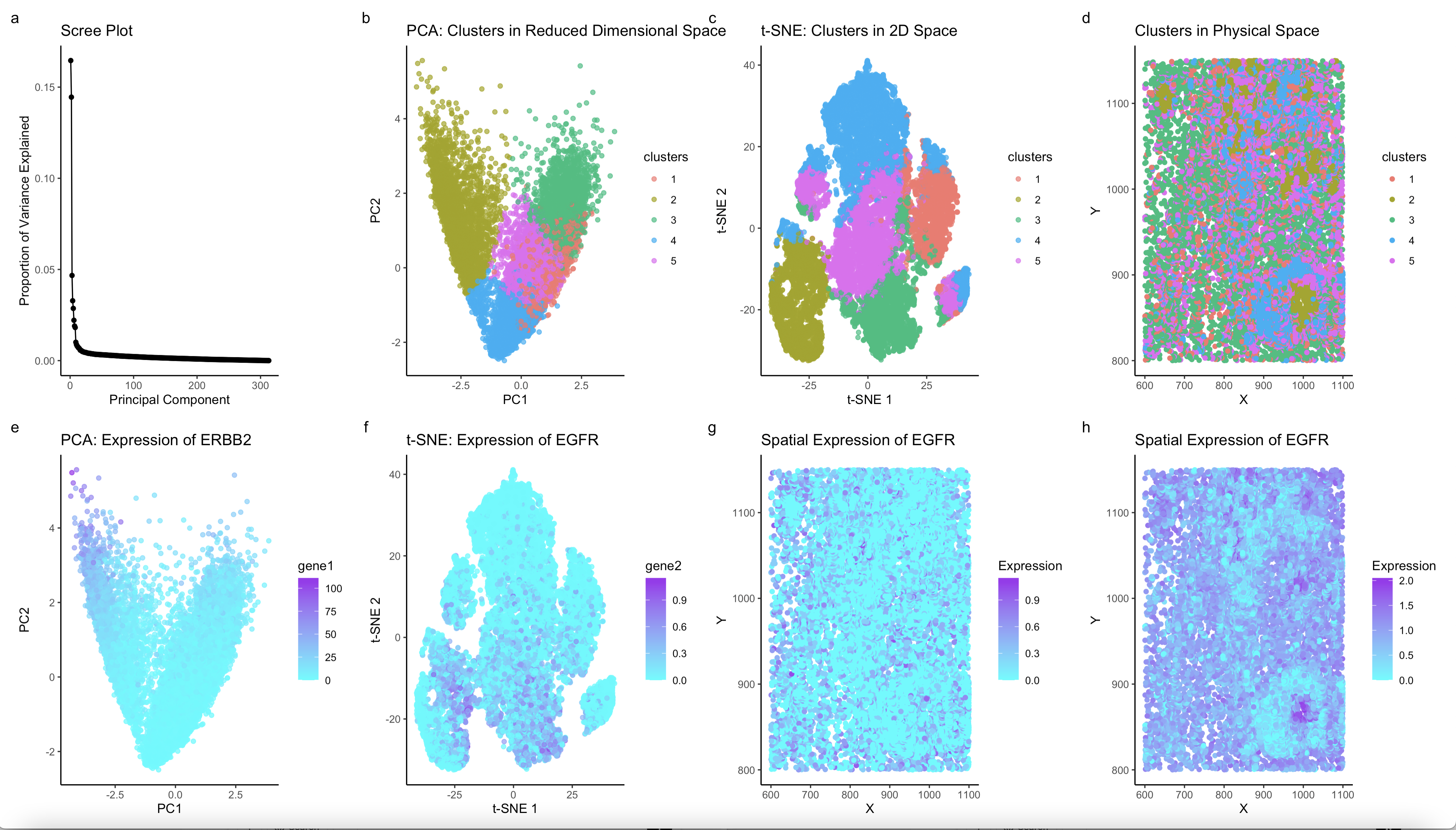
The figure I created presents an analysis of cell clustering and gene expression patterns using both dimensionality reduction techniques and spatial visualization. The scree plot (a) demonstrates that the first few principal components capture most of the variance, justifying the use of PCA and t-SNE for clustering. PCA (b) reveals distinct transcriptional clusters, with the olive-colored cluster appearing as a unique population. t-SNE (c) further refines this distinction by preserving local relationships, confirming that the olive cluster is not an artifact of linear variance but rather a biologically distinct group. The physical space clustering (d) shows that this cluster is not randomly distributed but instead occupies specific regions within the tissue, suggesting an organized spatial structure. The expression of ERBB2 (e) in PCA space highlights that this gene is predominantly upregulated in a specific population, aligning with the olive cluster. Similarly, the t-SNE visualization of EGFR expression (f) shows a matching pattern, reinforcing the co-expression of these genes. In the physical space plots (g, h), EGFR expression is localized and non-random, further supporting the hypothesis that the olive cluster corresponds to a distinct epithelial cell population. The strong co-expression of ERBB2 and EGFR, both in reduced and physical space, suggests that this cluster represents luminal epithelial cells, particularly those involved in active growth and signaling. These genes are hallmark markers of epithelial cell identity and proliferation, with established roles in tissue development, repair, and oncogenic transformation. Given their spatial localization and transcriptional profile, the olive cluster is likely composed of epithelial cells engaged in growth factor signaling, potentially representing a proliferative niche within the tissue.
To further validate this interpretation, I examined other genes known to co-express with ERBB2 and EGFR in epithelial cell populations. CDH1 (E-cadherin) and FOXA1, both critical regulators of epithelial identity and differentiation, showed similar spatial and transcriptional distributions. CDH1 is essential for maintaining cell-cell adhesion in epithelial tissues, while FOXA1 is a key transcription factor governing luminal epithelial lineage commitment. Their overlapping expression with ERBB2 and EGFR strengthens the hypothesis that the olive cluster represents luminal epithelial cells with an active role in tissue maintenance or regeneration. This co-expression pattern aligns with previous findings on epithelial lineage specification in glandular tissues, particularly in breast and lung epithelium, where ERBB2, EGFR, and FOXA1 interact to regulate cell fate (Jozwik & Carroll, 2012, Nat Rev Cancer DOI: 10.1038/nrc3262; van Roy & Berx, 2008, Cell Mol Life Sci DOI: 10.1007/s00018-008-8281-1).
2. Code (paste your code in between the ``` symbols)
1
2
3
4
5
6
7
8
9
10
11
12
13
14
15
16
17
18
19
20
21
22
23
24
25
26
27
28
29
30
31
32
33
34
35
36
37
38
39
40
41
42
43
44
45
46
47
48
49
50
51
52
53
54
55
56
57
58
59
60
61
62
63
64
65
66
67
68
69
70
71
72
73
74
75
76
77
78
79
80
81
82
83
84
85
86
87
88
89
90
91
92
93
94
95
96
97
98
99
100
101
102
103
104
105
106
107
108
109
110
111
112
113
114
115
116
117
118
119
120
121
122
123
124
125
126
127
128
129
130
131
132
133
134
# Load libraries
library(Rtsne)
library(ggplot2)
library(patchwork)

# Load Data
file <- '~/code/genomic-data-visualization-2025/data/pikachu.csv.gz'
data <- read.csv(file)

# Extract Position & Gene Expression Data
pos <- data[, 5:6]
rownames(pos) <- data$cell_id
gexp <- data[, 7:ncol(data)]
rownames(gexp) <- data$barcode

# Log Transformation of Gene Expression
gexp_log <- log10(gexp + 1)

# K-Means Clustering
set.seed(123)
clusters <- kmeans(gexp_log, centers=5)$cluster
clusters <- as.factor(clusters)
names(clusters) <- rownames(gexp)

# PCA
pcs <- prcomp(gexp_log)
df_pca <- data.frame(pcs$x, clusters)

# t-SNE using top PCs
set.seed(123)
tsne_emb <- Rtsne(pcs$x[, 1:10], dims = 2, perplexity = 50)$Y
df_tsne <- data.frame(tsne_emb, clusters)
names(df_tsne) <- c("X1", "X2", "clusters")

# Scree Plot (Variance Explained)
variance_explained <- pcs$sdev^2
total_variance <- sum(variance_explained)
proportion_variance_explained <- variance_explained / total_variance
pc_data <- data.frame(PC_Number = 1:length(proportion_variance_explained),
                      ProportionVariance = proportion_variance_explained)

p_scree <- ggplot(pc_data, aes(x = PC_Number, y = ProportionVariance)) +
  geom_line() +
  geom_point() +
  labs(title = "Scree Plot", x = "Principal Component", y = "Proportion of Variance Explained") +
  theme_classic()

# PCA - Cluster Visualization
p_pca_clusters <- ggplot(df_pca, aes(x=PC1, y=PC2, col=clusters)) +
  geom_point(alpha=0.7) +
  labs(title='PCA: Clusters in Reduced Dimensional Space', x="PC1", y="PC2") +
  theme_classic()

# t-SNE - Cluster Visualization
p_tsne_clusters <- ggplot(df_tsne, aes(x=X1, y=X2, col=clusters)) +
  geom_point(alpha=0.7) +
  labs(title='t-SNE: Clusters in 2D Space', x="t-SNE 1", y="t-SNE 2") +
  theme_classic()

# Physical Space - Cluster Visualization
p_physical_space <- ggplot(data) +
  geom_point(aes(x = aligned_x, y = aligned_y, col = clusters)) +
  labs(title = 'Clusters in Physical Space', x = "X", y = "Y") +
  theme_classic()

# Differential Expression for Specific Genes
gene_interest1 <- 'ERBB2'
df_pca$gene1 <- gexp[, gene_interest1]

p_gene_pca <- ggplot(df_pca, aes(x=PC1, y=PC2, col=gene1)) +
  geom_point(alpha=0.7) +
  labs(title=paste('PCA: Expression of', gene_interest1), x="PC1", y="PC2") +
  scale_color_gradient(low = "cyan", high = "purple") +
  theme_classic()

# t-SNE Expression Visualization for Other Genes
df_tsne$gene2 <- gexp_log[, 'EGFR']
p_gene_tsne1 <- ggplot(df_tsne, aes(x=X1, y=X2, col=gene2)) +
  geom_point(alpha=0.7) +
  labs(title='t-SNE: Expression of EGFR', x="t-SNE 1", y="t-SNE 2") +
  scale_color_gradient(low = "cyan", high = "purple") +
  theme_classic()

p_gene_space1 <- ggplot(data) +
  geom_point(aes(x = aligned_x, y = aligned_y, col = gexp_log[, 'ERBB2'])) +
  scale_color_gradient(low = "cyan", high = "purple") +
  labs(title = paste('Spatial Expression of', 'EGFR'),
       x = "X", y = "Y", color = "Expression") +
  theme_classic()

p_gene_space2 <- ggplot(data) +
  geom_point(aes(x = aligned_x, y = aligned_y, col = gexp_log[, 'EGFR'])) +
  scale_color_gradient(low = "cyan", high = "purple") +
  labs(title = paste('Spatial Expression of', 'EGFR'),
       x = "X", y = "Y", color = "Expression") +
  theme_classic()

# Combine Plots
combined_plot <- p_scree + p_pca_clusters + p_tsne_clusters + p_physical_space +
  p_gene_pca + p_gene_tsne1 + p_gene_space2 + p_gene_space1 +
  plot_annotation(tag_levels = 'a') +
  plot_layout(ncol = 4)

print(combined_plot)

# I want to try to find the top genes in the olive clster
olive_cluster_cells <- rownames(df_pca[df_pca$clusters == "1", ])
olive_cluster_expression <- colMeans(gexp_log[olive_cluster_cells, ])
other_clusters_expression <- colMeans(gexp_log[-which(rownames(gexp_log) %in% olive_cluster_cells), ])
log2fc <- log2(olive_cluster_expression + 1) - log2(other_clusters_expression + 1)
top_olive_genes <- sort(log2fc, decreasing = TRUE)[1:20]  # Top 20 most overexpressed genes
print(top_olive_genes)
#FCER1G

#those genes in the olive cluster with most variability compared to other clusters
olive_cluster_cells <- rownames(df_pca[df_pca$clusters == "1", ])  # Adjust if needed
var_olive <- apply(gexp_log[olive_cluster_cells, ], 2, var)
other_cells <- setdiff(rownames(gexp_log), olive_cluster_cells)
var_other <- apply(gexp_log[other_cells, ], 2, var)
var_ratio <- var_olive / (var_other + 1e-6)
top_variable_genes <- names(sort(var_ratio, decreasing = TRUE))[1:20]  # Top 20 most variable genes
print(top_variable_genes)


# ggplot(data) +
#   geom_point(aes(x = aligned_x, y = aligned_y, col = gexp_log[, 'FOXA1'])) +
#   scale_color_gradient(low = "cyan", high = "purple") +
#   labs(title = paste('Spatial Expression of', top_variable_genes[14]),
#        x = "X", y = "Y", color = "Expression") +
#   theme_classic()

#EGFR, CDH1, FOXA1, ERBB2