Analysis of Cell Type in Breast Cancer Tissue

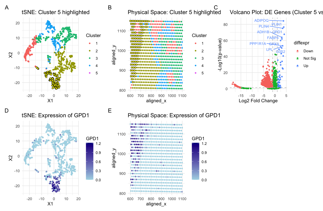
Based on my clustering analysis and differential expression testing, I identified GPD1 (Glycerol-3-Phosphate Dehydrogenase 1) as the most upregulated gene in Cluster 5, distinguishing it from all other clusters. The visualizations strongly suggest that this cluster represents a metabolically distinct population within the breast tissue sample. Panel A displays the tSNE space, with cluster 5 highlighted in yellow, indicating its separation from other clusters. Panel B maps these cells onto the physical space of the tissue, showing that they are concentrated in a specific region. Panel C, the volcano plot, reveals that GPD1 is one of the most highly upregulated genes in this cluster, with significant log₂ fold-change and statistical significance. Panels D and E demonstrate that GPD1 expression is enriched in cluster 5 in both reduced-dimensional (tSNE) and spatial coordinates. The strong upregulation of GPD1, along with other genes like ADIPOQ (Adiponectin) and FABP4 (Fatty Acid Binding Protein 4), suggests that cluster 5 consists of adipocyte-like or lipid-metabolizing cells. These genes are known markers of adipocytes, which are specialized cells responsible for fat storage and play key roles in metabolism and signaling within breast tissue.
Recent studies suggest that GPD1 functions as a tumor suppressor in breast cancer, influencing lipid metabolism through the PI3K/AKT signaling pathway (Xia et al., 2023). GPD1 overexpression has been shown to inhibit breast cancer cell proliferation, migration, and invasion, and higher levels of this gene correlate with better survival rates in breast cancer patients. Additionally, ADIPOQ, another gene highly expressed in this cluster, has been shown to induce autophagy-mediated apoptosis in breast cancer cells by activating the STK11/LKB1-AMPK-ULK1 pathway, ultimately suppressing tumor growth (Chung et al., 2017). This suggests that cluster 5 may represent a population of adipocytes or lipid-associated stromal cells that could help suppress breast cancer progression. Adipocytes are known to interact with breast cancer cells, influencing tumor behavior through metabolic and inflammatory signaling (Sierra et al., 2011). While adipocytes have been linked to both tumor-promoting and tumor-suppressing effects, the high expression of GPD1 and ADIPOQ in this cluster suggests that these cells may play a protective role in the tumor microenvironment by regulating lipid metabolism and promoting anti-cancer pathways.
Xia et al., 2023: https://www.ncbi.nlm.nih.gov/pmc/articles/PMC10362286/ Chung et al., 2017: https://pubmed.ncbi.nlm.nih.gov/28696138/ Sierra et al., 2011: https://pubmed.ncbi.nlm.nih.gov/22015313/
5. Code
1
2
3
4
5
6
7
8
9
10
11
12
13
14
15
16
17
18
19
20
21
22
23
24
25
26
27
28
29
30
31
32
33
34
35
36
37
38
39
40
41
42
43
44
45
46
47
48
49
50
51
52
53
54
55
56
57
58
59
60
61
62
63
64
65
66
67
68
69
70
71
72
73
74
75
76
77
78
79
80
81
82
83
84
85
86
87
88
89
90
91
92
93
94
95
96
97
98
99
100
101
102
103
104
105
106
107
108
109
110
111
112
113
114
115
116
117
118
119
120
121
122
123
124
125
126
127
128
129
130
131
132
133
134
135
136
# inspired by code-lesson-8
# libraries
library(ggplot2)
library(Rtsne)
library(patchwork)
library(ggrepel)

file <- "/Users/kevinnguyen/Desktop/genomic-data-visualization-2025/data/eevee.csv.gz"
data <- read.csv(file, row.names = 1)
head(data[1:5, 1:10])

# Extract physical coordinates.
pos <- data[, c("aligned_x", "aligned_y")]

# Extract gene expression data
gexp <- data[, 4:ncol(data)]

# Normalize: scale by library size then log10-transform (add 1 to avoid log(0))
totals <- rowSums(gexp)
norm_gexp <- gexp / totals * median(totals)
loggexp <- log10(norm_gexp + 1)

# Perform k-means clustering with 5 clusters (using 5 centers)
set.seed(2025)
km_out <- kmeans(loggexp, centers = 5)
clusters <- as.factor(km_out$cluster)
names(clusters) <- rownames(loggexp)

# Dimensionality reduction: PCA on log-transformed data, then tSNE on the first 10 PCs
pcs <- prcomp(loggexp)
tsne_res <- Rtsne(pcs$x[, 1:10])
tsne_df <- data.frame(X1 = tsne_res$Y[, 1],
                      X2 = tsne_res$Y[, 2],
                      clusters = clusters)

# Select cluster "5"
cluster_of_interest <- "5"
cat("Selected cluster of interest:", cluster_of_interest, "\n")

# Differential Expression Analysis: compare cluster 5 vs. all others using Wilcoxon test
cells_interest <- names(clusters)[clusters == cluster_of_interest]
cells_others <- names(clusters)[clusters != cluster_of_interest]

de_pvals <- sapply(colnames(gexp), function(gene) {
  wilcox.test(loggexp[cells_interest, gene],
              loggexp[cells_others, gene],
              alternative = "two.sided")$p.value
})
names(de_pvals) <- colnames(gexp)

# Compute log2 fold-change (using raw expression values) for each gene
log2fc <- sapply(colnames(gexp), function(gene) {
  mean_in <- mean(gexp[cells_interest, gene])
  mean_out <- mean(gexp[cells_others, gene])
  log2((mean_in + 1e-6) / (mean_out + 1e-6))
})
names(log2fc) <- colnames(gexp)

# Create a data frame for the volcano plot
volcano_df <- data.frame(gene = colnames(gexp),
                         log2FC = log2fc,
                         negLogP = -log10(de_pvals))
# Annotate significance
volcano_df$diffexpr <- "Not Sig"
volcano_df$diffexpr[volcano_df$log2FC > 1 & de_pvals < 0.05] <- "Up"
volcano_df$diffexpr[volcano_df$log2FC < -1 & de_pvals < 0.05] <- "Down"

# Label genes in the volcano plot: select the top 10 most significant
sig_genes <- volcano_df[de_pvals < 0.05 & abs(volcano_df$log2FC) > 1, ]
top_labels <- head(sig_genes[order(-sig_genes$negLogP), ], 10)
volcano_df$label <- NA
volcano_df$label[volcano_df$gene %in% top_labels$gene] <- volcano_df$gene[volcano_df$gene %in% top_labels$gene]

# Identify the gene most upregulated in the cluster
up_genes <- volcano_df[volcano_df$log2FC > 1 & de_pvals < 0.05, ]
if(nrow(up_genes) > 0) {
  up_gene <- up_genes$gene[which.max(up_genes$log2FC)]
} else {
  up_gene <- names(sort(log2fc, decreasing = TRUE))[1]
}
cat("Gene most upregulated in cluster", cluster_of_interest, ":", up_gene, "\n")

# Add gene-specific expression to the tSNE and spatial data
tsne_df$gene_expr <- loggexp[, up_gene]
pos_df <- data.frame(pos, clusters = clusters)
pos_df$gene_expr <- loggexp[, up_gene]

# Panel A: tSNE plot with the cluster of interest highlighted
p1 <- ggplot(tsne_df, aes(x = X1, y = X2)) +
  geom_point(aes(color = clusters), size = 1) +
  geom_point(data = tsne_df[clusters == cluster_of_interest, ],
             color = "black", size = 1.5, shape = 21, fill = "yellow") +
  labs(title = paste("tSNE: Cluster", cluster_of_interest, "highlighted"),
       color = "Cluster") +
  theme_minimal()

# Panel B: Physical space plot with the cluster of interest highlighted
p2 <- ggplot(pos_df, aes(x = aligned_x, y = aligned_y)) +
  geom_point(aes(color = clusters), size = 1) +
  geom_point(data = pos_df[clusters == cluster_of_interest, ],
             color = "black", size = 1.5, shape = 21, fill = "yellow") +
  labs(title = paste("Physical Space: Cluster", cluster_of_interest, "highlighted"),
       color = "Cluster") +
  theme_minimal()

# Panel C: Volcano plot
p3 <- ggplot(volcano_df, aes(x = log2FC, y = negLogP, color = diffexpr)) +
  geom_point(size = 1) +
  geom_text_repel(aes(label = label), size = 3, max.overlaps = Inf) +
  geom_vline(xintercept = c(-1, 1), linetype = "dashed", color = "gray") +
  geom_hline(yintercept = -log10(0.05), linetype = "dashed", color = "gray") +
  labs(title = paste("Volcano Plot: DE Genes (Cluster", cluster_of_interest, "vs Others)"),
       x = "Log2 Fold Change", y = "-Log10(p-value)") +
  theme_minimal()

# Panel D: tSNE plot colored by expression of the most upregulated gene (up_gene)
p4 <- ggplot(tsne_df, aes(x = X1, y = X2)) +
  geom_point(aes(color = gene_expr), size = 1) +
  scale_color_gradient(low = "lightblue", high = "darkblue") +
  labs(title = paste("tSNE: Expression of", up_gene),
       color = up_gene) +
  theme_minimal()

# Panel E: Physical space plot colored by expression of the most upregulated gene (up_gene)
p5 <- ggplot(pos_df, aes(x = aligned_x, y = aligned_y)) +
  geom_point(aes(color = gene_expr), size = 1) +
  scale_color_gradient(low = "lightblue", high = "darkblue") +
  labs(title = paste("Physical Space: Expression of", up_gene),
       color = up_gene) +
  theme_minimal()

# Plot
combined_plot <- p1 + p2 + p3 + p4 + p5 + plot_annotation(tag_levels = 'A')
print(combined_plot)