Interrogating Spatial Spot Cluster Differential Gene Expression with 10x Visium

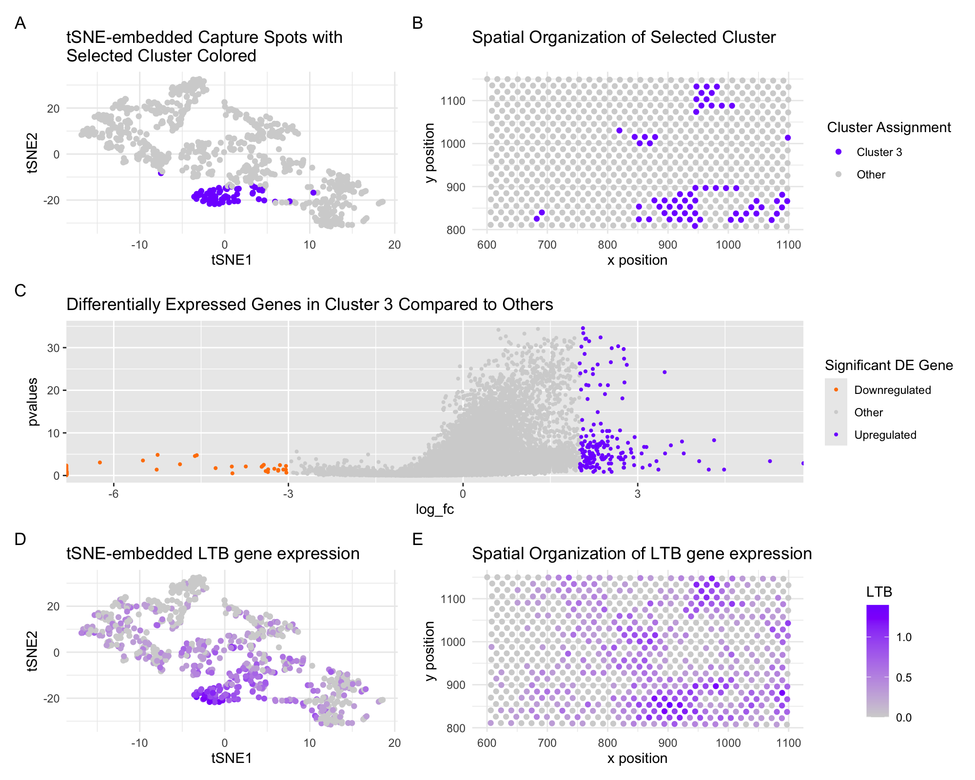
In these panels, I am depicting the representation of a 10x visium dataset in latent tSNE-embedded space and over the original spatial slide coordinates. I select a cluster based on the tSNE-embedded space (A) and visualize the spatial organization of the same cluster of spots on the spatial array (B). I then use the Wilcox test and compute fold change for each gene in the selected cluster 3 with respect to the same gene expression levels across the rest of the spot gene expression data. This differential gene expression is expressed as a function of magnitude of differential (fold change) and significance of the differential (p-value) and is shown illustrated in a volcano plot, with significant hits colored on the extreme right and left of the plot (C). From this plot, I select the gene LTB, and visualize corresponding normalized expression of LTB across the tSNE-embedded space and over spatial coordinates. LTB (lymphotoxin beta) encodes a protein that plays a crucial role in the immune system and inflammation, and as the significance of this hit would suggest, it is heavily correlated with cluster 3 phenotype. I conclude that the selected cluster 3 is likely an immune-related cell type– either T cells, B cells, or dendritic cells. Functionally, LTB anchors lymphotoxin-alpha to the surface of cells to mediate lymphotoxic activity. Further interrogation yields a similar expression pattern of CD4, reinforcing this conclusion.
1.https://www.ncbi.nlm.nih.gov/gene/4050#:~:text=Lymphotoxin%20beta%20is%20a%20type,Long%20Non%2DCoding%20RNA%20AL928768.
- https://www.uniprot.org/uniprotkb/Q06643/entry
- https://www.proteinatlas.org/ENSG00000227507-LTB
5. Code (paste your code in between the ``` symbols)
1
2
3
4
5
6
7
8
9
10
11
12
13
14
15
16
17
18
19
20
21
22
23
24
25
26
27
28
29
30
31
32
33
34
35
36
37
38
39
40
41
42
43
44
45
46
47
48
49
50
51
52
53
54
55
56
57
58
59
60
61
62
63
64
65
66
67
68
69
70
71
72
73
74
75
76
77
78
79
80
81
82
83
84
85
86
87
88
89
90
91
92
93
94
95
96
97
98
99
100
101
102
103
104
105
106
107
108
109
110
111
112
113
114
115
116
117
118
119
120
121
122
123
124
125
126
127
128
129
130
131
132
133
134
135
136
137
138
139
140
141
142
143
144
145
146
147
148
149
150
151
152
153
154
155
156


## SV Kammula | HW4

data <- read.csv('eevee.csv.gz')

library(ggplot2)
library(patchwork)
library(Rtsne)
library(ggrepel)

pos <- data[, 3:4]
rownames(pos) <- data$X
gexp <- data[, 5:ncol(data)]

norm <- gexp/rowSums(gexp) * 10000
rowSums(norm)
topgenes <- names(sort(colSums(norm), decreasing=TRUE)[1:1000])
normsub <- norm[,topgenes]

loggexp <- log10(gexp + 1)
com <- kmeans(loggexp, centers = 6)
clusters <- com$cluster
clusters <- as.factor(clusters)
names(clusters) <- rownames (gexp)
head(clusters)

pcs <- prcomp(loggexp)
df <- data.frame(pcs$x, clusters, gene = gexp[, 'CD4'])
ggplot(df, aes(x=PC1, y=PC2, col=clusters)) + geom_point()


## embedding

emb <- Rtsne::Rtsne(pcs$x[,1:10])$Y
head(emb)

df <- data.frame(emb, clusters, gene = loggexp[, 'LTB'])
ggplot(df, aes(x=X1, y=X2, col=clusters)) + geom_point()

# choose cluster 3; look at CD4
df$clusters_colored <- ifelse(df$clusters == 3, "Cluster 3", "Other")


# panel 1
g1 <- ggplot(df, aes(x = X1, y = X2, col = clusters_colored)) +
  geom_point() +
  scale_color_manual(values = c("Cluster 3" = "#8000FF", "Other" = "lightgray")) +
  labs(color = "Cluster Assignment") +
  theme_minimal() +
  ggtitle('tSNE-embedded Capture Spots with \nSelected Cluster Colored') +
  xlab("tSNE1") +
  ylab("tSNE2") +
  theme(legend.position = "none")


# panel 2
g2 <- ggplot(pos, aes(x = aligned_x, y = aligned_y, col = df$clusters_colored)) +
  geom_point() +
  scale_color_manual(values = c("Cluster 3" = "#8000FF", "Other" = "lightgray")) +
  labs(color = "Cluster Assignment") +
  ggtitle('Spatial Organization of Selected Cluster') +
  theme_minimal() +
  xlab("x position") +
  ylab("y position")


# panel 3
g4 <- ggplot(df, aes(x = X1, y = X2, col = gene)) +
  geom_point() +
  scale_color_gradient(high = "#8000FF", low = "lightgray") +
  labs(color = 'LTB') +
  theme_minimal() +
  ggtitle('tSNE-embedded LTB gene expression') +
  xlab("tSNE1") +
  ylab("tSNE2") +
  theme(legend.position = "none")


# panel 4
g5 <- ggplot(pos, aes(x = aligned_x, y = aligned_y, col = df$gene)) +
  geom_point() +
  scale_color_gradient(high = "#8000FF", low = "lightgray") +
  labs(color = 'LTB') +
  ggtitle('Spatial Organization of LTB gene expression') +
  theme_minimal() +
  xlab("x position") +
  ylab("y position")


interest <- 3
cellsOfInterest <- names(clusters)[clusters == interest]
otherCells <- names(clusters)[clusters != interest]
i <- 'CD4' #find on expressed in cluster of interest
genetest <- norm[,i]
names(genetest) <- rownames(norm)
genetest[cellsOfInterest]
genetest[otherCells]
t.test(genetest[cellsOfInterest], genetest[otherCells], )


# differential gene expression
pvalues <- sapply(colnames(norm), function(i) {
  wilcox.test(gexp[clusters == 3, i], gexp[clusters != 3, i])$p.val
})

# get log fold change
logfc <- sapply(colnames(gexp), function(i) {
  log2(mean(norm[clusters == 3, i])/mean(norm[clusters != 3, i]))
})

valid_indices <- !is.na(pvalues)
filtered_pvalues = pvalues[valid_indices]
filtered_logfc = logfc[valid_indices]


# volcano plot
df_volc = data.frame(pvalues = -log10(filtered_pvalues), log_fc = filtered_logfc)
df_volc$genes <- rownames(df_volc)


#df_volc_cleaned <- df_volc[!is.nan(df_volc$p_values) & !is.nan(df_volc$logFC), ]
upper_logfc <- 2
lower_logfc <- -3

df_volc$color <- ifelse(df_volc$log_fc > upper_logfc, "Upregulated",
                  ifelse(df_volc$log_fc < lower_logfc, "Downregulated", "Other"))


g3 <- ggplot(df_volc, aes(x = log_fc, y = pvalues, color = color)) +
  geom_point(size= 0.75) +
  ggtitle("Differentially Expressed Genes in Cluster 3 Compared to Others") +
  scale_color_manual(values = c("Upregulated" = "#8000FF",
                                "Downregulated" = "#FF8000",
                                "Other" = "lightgray")) +
  labs(color = "Significant DE Gene")
  #scale_color_manual(values = c("Cluster 3" = "#8000FF", "Other" = "lightgray")) +
  xlab("log2(FC)") +
  ylab("-log10(p-value)")


(g1 + g2) / g3 / (g4 + g5) + plot_annotation(tag_levels = 'A')


###