HW3: Exploring Cell Type with Differentially upregulated CD52

1. Figure Description.
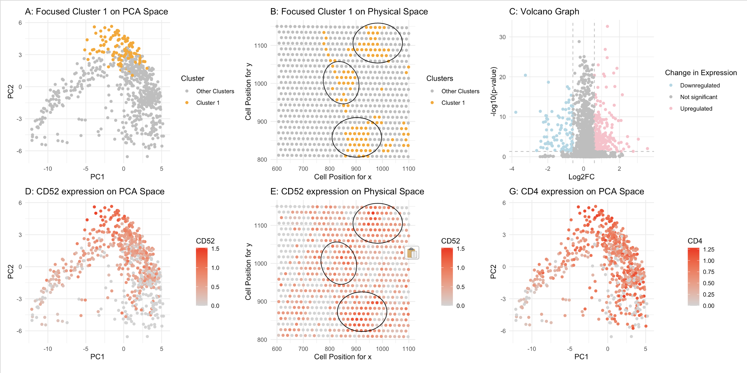
Figure A: Cluster 1 is highlighted in orange in PCA space, while the remaining six clusters are shown in grey. The axes represent PC1 and PC2. Figure B: Cluster 1 is highlighted in orange to show its distribution in physical space, with the remaining six clusters in grey. The axes represent x and y spot positions. Figure C: A volcano plot comparing gene expression in Cluster 1 versus the other clusters. The y-axis represents p-values in -log10 scale, while the x-axis represents log2 fold changes between Cluster 1 and the rest of the clusters. Figure D: CD52 gene expression is visualized in PCA space, highlighted in a gradient red. Figure E: CD52 gene expression is visualized in physical space, highlighted in a gradient red. Figure G: CD4 gene expression is visualized in PCA space, highlighted in a gradient red.
2. Cluster interpretation.
Cluster 1 spots show differentially upregulated CD52. We know this because, in Figures A and D, Cluster 1 has the highest CD52 gene expression level in PCA space. This is also evident in Figures B and E, where spots in Cluster 1 exhibit a high expression level of CD52 in physical space. The cell marker CD52 is commonly found in mature lymphocytes, natural killer (NK) cells, eosinophils, neutrophils, monocytes/macrophages, and dendritic cells (DCs). Therefore, Cluster 1 likely belongs to one of these populations. Additionally, CD4, a marker for helper T cells, is also differentially upregulated in Cluster 1. Combining these two markers, it is reasonable to assume that Cluster 1 represents helper T cells.
3. Citation.
https://pubmed.ncbi.nlm.nih.gov/28283679/#:~:text=Introduction%3A%20CD52%20(Campath%2D1,and%20dendritic%20cells%20(DCs).
https://clinicalinfo.hiv.gov/en/glossary/cd4-t-lymphocyte#:~:text=A%20type%20of%20lymphocyte.,cells)%2C%20to%20fight%20infection.
4. Code
1
2
3
4
5
6
7
8
9
10
11
12
13
14
15
16
17
18
19
20
21
22
23
24
25
26
27
28
29
30
31
32
33
34
35
36
37
38
39
40
41
42
43
44
45
46
47
48
49
50
51
52
53
54
55
56
57
58
59
60
61
62
63
64
65
66
67
68
69
70
71
72
73
74
75
76
77
78
79
80
81
82
83
84
85
86
87
88
89
90
91
92
93
94
95
96
97
98
99
100
101
102
103
104
105
106
107
108
109
110
111
112
113
114
115
116
117
118
119
120
121
122
123
124
125
126
127
128
129
130
library(ggplot2)
library(patchwork)

file <- '"~/Downloads/eevee.csv.gz"'
data <- read.csv(file)
data[1:5,1:10]

pos <- data[, 3:4]
rownames(pos) <- data$cell_id
gexp <- data[, 5:ncol(data)]
rownames(gexp) <- data$barcode
head(gexp)
head(pos)

gexp[1:5, 1:10]
dim(gexp)

# limiting to top 1000 most highly expressed genes
topgenes <- names(sort(colSums(gexp), decreasing=TRUE)[1:2000])
gexpsub <- gexp[,topgenes]
gexpsub[1:5,1:5]
dim(gexpsub)

# normalization
norm <- gexpsub/rowSums(gexpsub) *10000
loggexp <- log10(norm+1)
dim(loggexp)

## kmeans
ks = 1:25
totw <- sapply(ks, function(k) {
  print(k)
  com <- kmeans(loggexp, centers=k)
  return(com$tot.withinss)
})
g1 <- plot(ks, totw)

# pick k = 7
com <- kmeans(loggexp, centers=7)
clusters <- com$cluster
clusters <- as.factor(clusters)
names(clusters) <- rownames(loggexp)
head(clusters)

# PCA
pcs <- prcomp(loggexp)
df <- data.frame(pcs$x,clusters)
ggplot(df, aes(x=PC1, y=PC2, col= clusters)) + geom_point()

g3<- ggplot(df, aes(x=PC1, y=PC2, col= factor(clusters==6, labels = c("Other Clusters","Cluster 1")))) +
              geom_point() +
              scale_color_manual(values = c("Cluster 1" = "orange", "Other Clusters" = "grey"))+
              labs(title = "A: Focused Cluster 1 on PCA Space", col = "Cluster") +
              theme_minimal()


df <- data.frame(pos,loggexp,clusters)
g4 <- ggplot(df, aes(x = aligned_x, y = aligned_y, col = factor(clusters==6, labels = c("Other Clusters","Cluster 1")))) +
              geom_point() +
              scale_color_manual(values = c("Cluster 1" = "orange", "Other Clusters" = "grey"))+
              labs(title = "B: Focused Cluster 1 on Physical Space", col = "Clusters",
                   x = "Cell Position for x",
                   y = "Cell Position for y") +
        theme_minimal()

g3 + g4

# differential expression
cellsOfInterest <- names(clusters)[clusters == 6]
otherCells <- names(clusters)[clusters != 6]

results <- sapply(1:ncol(gexpsub), function(i) {
  genetest <- gexpsub[,i]
  names(genetest) <- rownames(gexpsub)
  out <- t.test(genetest[cellsOfInterest], genetest[otherCells], alternative = 'greater')
  out$p.value
})

names(results) <- colnames(gexpsub)
results <- sort(results, decreasing = FALSE)
length(results)


Cluster1Cell <- gexpsub[cellsOfInterest,]
SumCluster1Cell <- colSums(Cluster1Cell)/length(cellsOfInterest)

OtherClustersCell <- gexpsub[otherCells,]
SumOtherClustersCell <- colSums(OtherClustersCell)/length(otherCells)

log_results <- results
log_2FC <- log2(SumCluster1Cell/SumOtherClustersCell)

ggplot(data.frame(log_results), aes(x = log_results))+
  geom_histogram(binwidth = 1, fill = "lightblue", color = "black", alpha = 0.7)+
  labs(title = "C: Histogram of -log10 Transformed p-values",
       x = "-log10(p-value)",
       y = "Frequency") +
       theme_minimal()

df <- data.frame(log_results, log_2FC)
df$diffexpressed <- "NO"
df$diffexpressed[df$log_2FC > 0.6 & df$log_results < (0.05)] <- "UP"
df$diffexpressed[df$log_2FC < -0.6 & df$log_results < (0.05)] <- "DOWN"

g5<- ggplot(df, aes(y=-log10(log_results), x = log_2FC, col = diffexpressed)) + geom_point() +
  geom_vline(xintercept = c(-0.6, 0.6), col = "gray", linetype = 'dashed') +
  geom_hline(yintercept = -log10(0.05), col = "gray", linetype = 'dashed') +
  labs(title = "C: Volcano Graph",
          y = "-log10(p-value)",
          x = "Log2FC", col = "Change in Expression") +
  scale_color_manual(values = c("lightblue", "grey", "pink"),
                     labels = c("Downregulated", "Not significant", "Upregulated"))+
  theme_minimal()

# one gene in PCA
df <- data.frame(pcs$x, clusters, gene = loggexp[, 'CD52'])
g6 <- ggplot(df, aes(x=PC1, y=PC2, col=gene)) + labs(title = "D: CD52 expression on PCA Space", col = "CD52") +
  scale_color_gradient(low = 'lightgrey', high = 'red') + geom_point() + theme_minimal()


# one gene in physical space
df <- data.frame(pos, gene = loggexp[,"CD52"])
g7 <- ggplot(df, aes(x = aligned_x, y = aligned_y, col = gene)) +
  labs(title = "E: CD52 expression on Physical Space ",
       x = "Cell Position for x",
       y = "Cell Position for y",
       col = "CD52") + scale_color_gradient(low = 'lightgrey', high = 'red') +
  geom_point() + theme_minimal()

g3 + g4 + g5 + g6 + g7