Rediscovering the Same Epithelial Cell Type in Spatial Transcriptomics: Leveraging ELF3 Expression Across Datasets

Validation of Same Cell Type
In my previous analysis of the Pikachu dataset, I identified a specific cell cluster characterized by the upregulation of ELF3, a well-established marker of epithelial cells. This cluster exhibited a distinct transcriptional profile that set it apart from other cell populations. For this assignment, I aimed to identify the same epithelial cell type within the Eevee dataset, which is based on spot-level spatial transcriptomics rather than single-cell resolution.
To establish the correspondence between the epithelial cell population in Pikachu and Eevee, I leveraged ELF3 expression as a means to locate the same cell type. The key evidence supporting this identification lies not only in the fact that ELF3 is upregulated in a distinct group of spots but also in the similarity of the spatial distribution of ELF3 expression and the clustering pattern in both datasets. That is, the overall structure of the ELF3-expressing group and its relationship to other transcriptional clusters are highly comparable between the two datasets, confirming that I have found the same cell type.
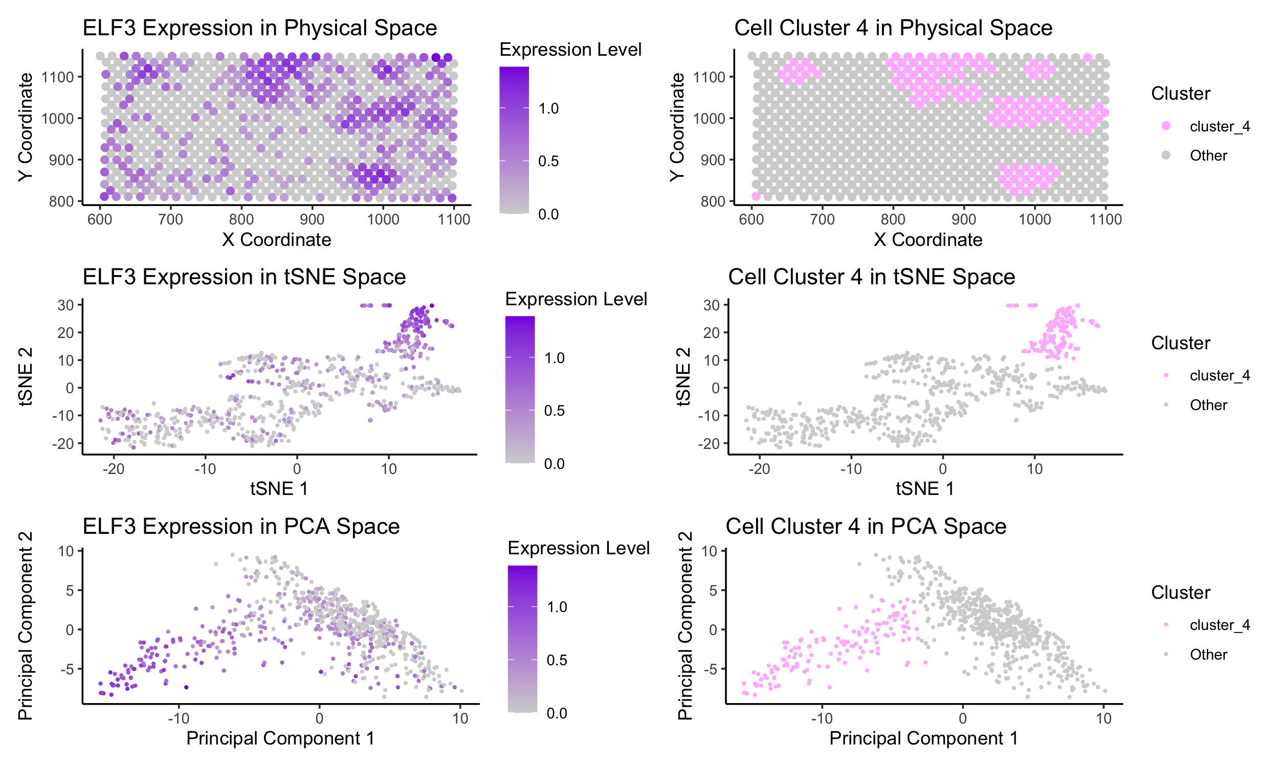
First, I examined ELF3 expression in the physical tissue space of the Eevee dataset (Panel A). The results revealed a coherent, spatially contiguous group of spots where ELF3 was highly expressed, mirroring the distribution observed in Pikachu. The fact that ELF3 expression is not randomly dispersed but instead forms a localized cluster in both datasets strongly suggests that these spots correspond to the same epithelial cell population rather than an artifact of dataset differences.
To further validate this identification, I applied dimensionality reduction techniques, including t-SNE (Panels C and D) and PCA (Panels E and F). In both analyses, the ELF3-expressing spots were concentrated within a well-defined region, just as they were in Pikachu. Importantly, the overall cluster structure in these reduced spaces was also highly similar, meaning that not only did ELF3-positive spots cluster together, but the surrounding clusters and their relationships to ELF3-expressing cells remained comparable across datasets. This reinforces the conclusion that I successfully rediscovered the same epithelial cell type, rather than merely detecting ELF3 expression in an unrelated group of cells.
Changes I have made
To refine my clustering approach and ensure robust identification of ELF3-expressing cells, I performed k-means clustering. Initially, I set k=10, but through analysis of the within-cluster variance (total within-cluster sum of squares), I determined that k=4 provided the most meaningful biological segmentation. This decision was based on the observation that higher k values led to oversegmentation, fragmenting transcriptionally coherent cell groups.
A key difference between the Pikachu and Eevee datasets is the resolution: Pikachu consists of single-cell data, whereas Eevee contains spatial spots, each potentially encompassing multiple cell types. This difference likely explains why the optimal number of clusters in Eevee is lower, as transcriptionally distinct populations are less granular in spot-level data. Nonetheless, the robust recurrence of an ELF3-expressing cluster across analyses strongly suggests that I have identified the same epithelial cell population in both datasets.
To improve data visualization and clarity, I made several refinements. I increased point sizes in scatter plots to enhance readability and modified axis labels and legends to ensure intuitive interpretation. These adjustments provide a clearer representation of ELF3-expressing cells and their spatial and transcriptional characteristics.
Conclusion
By leveraging ELF3 as a marker, analyzing its spatial and transcriptional distribution, and refining clustering approaches, I successfully identified the same epithelial cell type in the Eevee dataset as in Pikachu. The consistency of ELF3 expression and cell clustering across multiple analytical techniques provides strong evidence that this cluster represents epithelial cells, supporting the validity of my findings.
Code (paste your code in between the ``` symbols)
1
2
3
4
5
6
7
8
9
10
11
12
13
14
15
16
17
18
19
20
21
22
23
24
25
26
27
28
29
30
31
32
33
34
35
36
37
38
39
40
41
42
43
44
45
46
47
48
49
50
51
52
53
54
55
56
57
58
59
60
61
62
63
64
65
66
67
68
69
70
71
72
73
74
75
76
77
78
79
80
81
82
83
84
85
86
87
88
89
90
91
92
93
94
95
96
97
98
99
100
101
102
103
104
105
106
107
108
109
110
111
112
113
114
115
116
117
118
119
120
121
122
123
124
125
126
127
128
129
# Load the data
data <- read.csv('~/Desktop/genomic_data_visualization/genomic-data-visualization-2025/data/eevee.csv.gz')

# Import libraries
library(ggplot2)
library(patchwork)
library(Rtsne)
library(ggrepel)

# Extract physical coordinates and gene expression data
pos = data[,2:3]
rownames(pos) <- data$barcode
gexp = data[,4:ncol(data)]
rownames(gexp) <- data$barcode

# Normalize and log-transform the gene expression data
gexpnorm <- log10(gexp/rowSums(gexp) * mean(rowSums(gexp)) + 1)

# Perform PCA
pcs <- prcomp(gexpnorm)
plot(pcs$sdev[1:30])

# Plot gene ELF3 in physical space
plot.df <- data.frame(aligned_x = data$aligned_x,
                      aligned_y = data$aligned_y,
                      ELF3 = gexpnorm[, "ELF3", drop = FALSE])

p1 <- ggplot(plot.df, aes(aligned_x, aligned_y, col=ELF3)) +
  geom_point(size=1.8) +
  theme_classic() +
  scale_color_gradient(low='lightgrey', high='blueviolet') +
  ggtitle("ELF3 Expression in Physical Space") +
  labs(x = "X Coordinate", y = "Y Coordinate", color = "Expression Level")

# Perform tSNE
tsne <- Rtsne(pcs$x[, 1:20])$Y
ggplot(data.frame(tsne)) + geom_point(aes(x = X1, y = X2), size = 0.5) + theme_classic()

# Plot gene ELF3 in tSNE space
plot.df <- data.frame(emb1 = tsne[,1],
                      emb2 = tsne[,2],
                      ELF3 = gexpnorm[, "ELF3", drop = FALSE])

p2 <- ggplot(plot.df, aes(emb1, emb2,col=ELF3)) +
  geom_point(size = 0.5) +
  theme_classic() +
  scale_color_gradient(low='lightgrey', high='blueviolet') +
  ggtitle("ELF3 Expression in tSNE Space") +
  labs(x = "tSNE 1", y = "tSNE 2", color = "Expression Level")

# Plot gene ELF3 in PCA space
plot.df <- data.frame(pcs$x,
                      ELF3 = gexpnorm[, "ELF3", drop = FALSE])

p3 <- ggplot(plot.df, aes(x = PC1, y = PC2, col = ELF3)) +
  geom_point(size = 0.5) +
  theme_classic() +
  scale_color_gradient(low='lightgrey', high='blueviolet') +
  ggtitle("ELF3 Expression in PCA Space") +
  labs(x = "Principal Component 1", y = "Principal Component 2", color = "Expression Level")

# Check total within-cluster to find optimal k
totw <- sapply(2:25, function(k) {
  com <- kmeans(tsne, centers = k)
  return(com$tot.withinss)
})
plot(2:25, totw, type = "b", pch = 19, col = "purple",
     xlab = "Number of Clusters (k)", ylab = "Total Within-Cluster Variance",
     main = "Total Within-Cluster Variance for Optimal k")

# Perform k-means clustering with chosen k = 5
kmeans_result <- kmeans(tsne, centers = 4)
clusters <- as.factor(kmeans_result$cluster)

# Look at all groups to choose one from
names(clusters) <- rownames(gexpnorm)
df <- data.frame(pcs$x, clusters)
ggplot(df, aes(x=PC1, y=PC2, col=clusters)) + geom_point(size=0.5)

# Define color for the chosen cluster
cluster.cols <- c("plum1", "lightgrey")
names(cluster.cols) <- c("cluster_4", "Other")
selected_cluster <- 4

# Create a new data frame for plotting in tSNE space
df_tsne <- data.frame(
  emb1 = tsne[, 1],
  emb2 = tsne[, 2],
  cluster = ifelse(kmeans_result$cluster == selected_cluster, "cluster_4", "Other")
)

# Plot cluster 4 in tSNE space
p4 <- ggplot(df_tsne, aes(x = emb1, y = emb2, col = cluster)) +
  geom_point(size = 0.5) +
  theme_classic() +
  scale_color_manual(values = cluster.cols) +
  ggtitle("Cell Cluster 4 in tSNE Space") +
  labs(x = "tSNE 1", y = "tSNE 2", color = "Cluster")

# Create a new data frame for plotting in PCA space
df_pca <- data.frame(pcs$x,
                     cluster = ifelse(kmeans_result$cluster == selected_cluster,
                                      "cluster_4", "Other"))

# Plot cluster 4 in PCA space
p5 <- ggplot(df_pca, aes(x = PC1, y = PC2, col = cluster)) +
  geom_point(size = 0.5) +
  theme_classic() +
  scale_color_manual(values = cluster.cols) +
  ggtitle("Cell Cluster 4 in PCA Space") +
  labs(x = "Principal Component 1", y = "Principal Component 2", color = "Cluster")

# Create a new data frame for plotting in physical space
df_phys <- data.frame(
  aligned_x = data$aligned_x,
  aligned_y = data$aligned_y,
  cluster = ifelse(kmeans_result$cluster == selected_cluster, "cluster_4", "Other")
)

# Plot cluster 4 in physical space
p6 <- ggplot(df_phys, aes(aligned_x, aligned_y, col = cluster)) +
  geom_point(size = 1.8) +
  theme_classic() +
  scale_color_manual(values = cluster.cols) +
  ggtitle("Cell Cluster 4 in Physical Space") +
  labs(x = "X Coordinate", y = "Y Coordinate", color = "Cluster")

# plot using patchwork
(p1 + p6) / (p2 + p4) / (p3 + p5)