Identifying the Same Cluster of Breast Granular Cells in the Pikachu Dataset

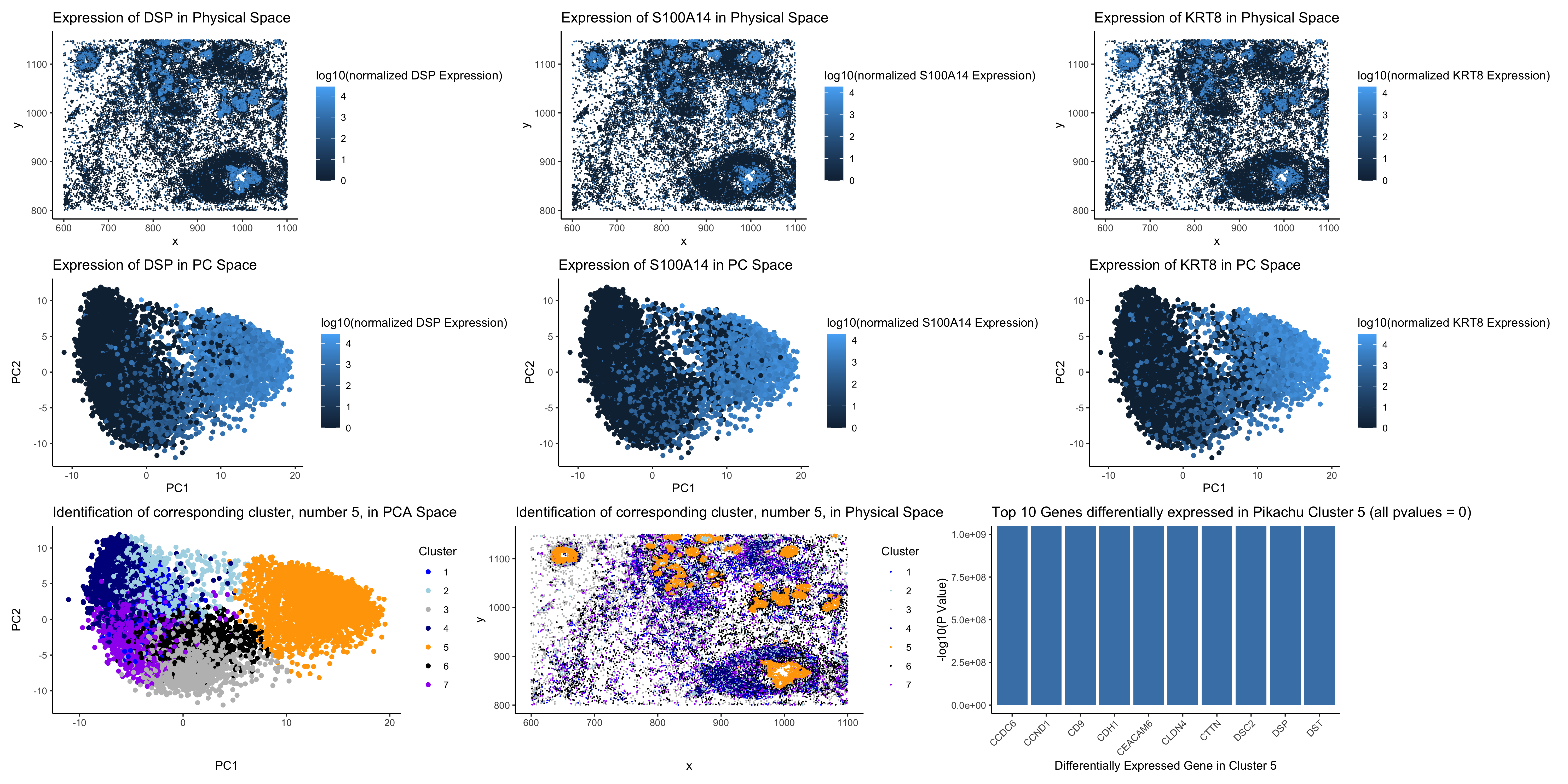
I found the same breast granular cell type that I identified in the Eevee dataset in the Pikachu dataset. To do so, I first identified the number of clusters to use in kmeans for the Pikachu dataset, which I found to be 7, the same number that I used in the Eevee dataset, by finding the elbow in the total withiness curve vs. k values. I also believe that keeping this number the same is beneficial to identifying the same cluster in a different dataset because it reduces the risk of the cluster being broken into subclusters in this analysis. I then visualized the location in both physical and reduced dimensional (PCA) space of the 3 most differentially expressed genes that I identified in the Eevee dataset. I then looked at the physical and reduced dimensional spread of the new clusters I had created in the Pikachu dataset and identified the cluster that aligned with the location of upregulation of these three genes in both physical and reduced dimensional space. Finally, I performed differential gene expression on that cluster as compared to the other clusters in the Pikachu set and researched the top 10 genes that were found. Two of the genes were the same as two of the genes in the top 10 differentially expressed genes from my identified cluster in the Eevee set, and all others were found to be expressed at high levels in the “breast granular cell” clusters from Protein Atlas that I used to identify my cell type for HW3 (https://www.proteinatlas.org/ENSG00000096696-DSP/single+cell/breast). Additionally, I tested a number of the other genes from the top 10 differentially expressed genes list form the Eevee cluster (the ones that were also in the Pikachu dataset) and found them all to be differentially expressed in the Pikachu cluster. Thus, I believe that I have identified the same cell-type in the Pikachu data that I identified in the Eevee dataset for HW3.
I changed my code from HW3 in a number of ways for this homework. I first set a seed in this code to ensure that my results are reproducible. Then, I changed the order in which I analyzed and visualized the data. I chose to begin with visualizing the genes I identified from the Eevee dataset in both physical and reduced dimensional space to see their alignment with the clusters I later generated in the Pikachu dataset, so that I could identify the correct cluster that corresponds with the Eevee cluster. I chose to include visualizations of this data for 3 genes, so that it was clear that I had identified the same cell type not just a population that shared 1 gene. Finally, I performed differential gene expression analysis at the end to confirm that these two clusters from the different datasets were in fact the same cell type. I also changed my visualization to include 9 panels given these extra visualizations. I had hoped to include a volcano plot but given that my p values were “0” for the 10 most differentially expressed genes, they would have been out of range of the graph.
1
2
3
4
5
6
7
8
9
10
11
12
13
14
15
16
17
18
19
20
21
22
23
24
25
26
27
28
29
30
31
32
33
34
35
36
37
38
39
40
41
42
43
44
45
46
47
48
49
50
51
52
53
54
55
56
57
58
59
60
61
62
63
64
65
66
67
68
69
70
71
72
73
74
75
76
77
78
79
80
81
82
83
84
85
86
87
88
89
90
91
92
93
94
95
96
97
98
99
100
101
102
103
104
105
106
107
108
109
110
111
112
113
114
115
116
117
118
119
120
121
122
123
124
125
126
127
128
129
130
131
132
133
134
135
136
137
138
139
install.packages('patchwork')
set.seed(1)

file <- '/Users/alexgorham/Desktop/genomic-data-visualization-2025/data/pikachu.csv.gz'
data <- read.csv(file)
head(data)

pos <- data[,5:6]
rownames(pos) <-data$barcode
gexp <- data[,7:ncol(data)]
rownames(gexp) <- data$barcode
area <- data[,3]

norm <- (gexp/area)*100000 #cell area normalization
norm
logexp <- log10(norm+1) #log on the normalized data
logexp

ks = c(1, 2, 3, 4, 5, 7, 9, 11, 13, 15, 17, 19, 21, 23, 25, 27, 29, 31, 33, 35)
totw <- sapply(ks, function(k) {
  print(k)
  com <- kmeans(logexp, centers = k) # using the log transformed data
  return(com$tot.withinss)
})
totw
plot(ks, totw)
# determined 7 clusters seems to be the elbow (same as for Eevee data)

pcs <- prcomp(logexp)
com <- kmeans(pcs$x[,1:15], centers = 7)
clusters <- com$cluster
names(clusters) <- rownames(gexp)
head(clusters)

library(ggplot2)
df5 <- data.frame(x = pos$aligned_x, y = pos$aligned_y, gene = logexp[,'DSP'])
panel5 <- ggplot(df5, aes(x=x, y = y, col = gene)) + geom_point(size = 0.1) +
  labs(title = "Expression of DSP in Physical Space",
       colour = 'log10(normalized DSP Expression)') +
  theme_classic()
panel5

df4 <- data.frame(pcs$x[,1:2], clusters, gene = logexp[,'DSP'])
panel4 <- ggplot(df4, aes(x=PC1, y = PC2, col = gene)) + geom_point() +
  labs(title = "Expression of DSP in PC Space",
       colour = 'log10(normalized DSP Expression)') +
  theme_classic()
panel4

df7 <- data.frame(x = pos$aligned_x, y = pos$aligned_y, gene = logexp[,'S100A14'])
panel7 <- ggplot(df7, aes(x=x, y = y, col = gene)) + geom_point(size = 0.1) +
  labs(title = "Expression of S100A14 in Physical Space",
       colour = 'log10(normalized S100A14 Expression)') +
  theme_classic()
panel7

df6 <- data.frame(pcs$x[,1:2], clusters, gene = logexp[,'S100A14'])
panel6 <- ggplot(df6, aes(x=PC1, y = PC2, col = gene)) + geom_point() +
  labs(title = "Expression of S100A14 in PC Space",
       colour = 'log10(normalized S100A14 Expression)') +
  theme_classic()
panel6

df9 <- data.frame(x = pos$aligned_x, y = pos$aligned_y, gene = logexp[,'KRT8'])
panel9 <- ggplot(df9, aes(x=x, y = y, col = gene)) + geom_point(size = 0.1) +
  labs(title = "Expression of KRT8 in Physical Space",
       colour = 'log10(normalized KRT8 Expression)') +
  theme_classic()
panel9

df8 <- data.frame(pcs$x[,1:2], clusters, gene = logexp[,'KRT8'])
panel8 <- ggplot(df8, aes(x=PC1, y = PC2, col = gene)) + geom_point() +
  labs(title = "Expression of KRT8 in PC Space",
       colour = 'log10(normalized KRT8 Expression)') +
  theme_classic()
panel8

df <- data.frame(pcs$x[,1:2], clusters)
panel1 <- ggplot(df, aes(x=PC1, y = PC2, col = factor(clusters))) + geom_point() +
  scale_color_manual(values = c('1' = 'blue',
                                '2' = 'lightblue',
                                '3' = 'grey',
                                '4' = 'darkblue',
                                '5' = 'orange',
                                '6' = 'black',
                                '7' = 'purple')) +
  labs(title = "Identification of corresponding cluster, number 5, in PCA Space",
       colour = 'Cluster') +
  theme_classic()
panel1

df2 <- data.frame(x = pos$aligned_x, y = pos$aligned_y, clusters)
panel2 <- ggplot(df2, aes(x=x, y = y, col = factor(clusters))) + geom_point(size = 0.1) +
  scale_color_manual(values = c('1' = 'blue',
                                '2' = 'lightblue',
                                '3' = 'grey',
                                '4' = 'darkblue',
                                '5' = 'orange',
                                '6' = 'black',
                                '7' = 'purple')) +
  labs(title = "Identification of corresponding cluster, number 5, in Physical Space",
       colour = 'Cluster') + theme_classic()
panel2

interest <- 5
cellsOfInterest <- names(clusters)[clusters == interest]
otherCells <- names(clusters)[clusters != interest]

results <- sapply(1:ncol(logexp), function(i){
  genetest <- logexp[,i]
  names(genetest) <- rownames(logexp)
  out <- t.test(genetest[cellsOfInterest], genetest[otherCells], alternative = 'greater')
  out$p.value
})
names(results) <- colnames(logexp)
names(sort(results, decreasing = FALSE)[1:100])
sort(results, decreasing = FALSE)

df3 <- data.frame(gene = names(sort(results, decreasing = FALSE)[1:10]), pval = sort(results, decreasing = FALSE)[1:10])
order <- names(sort(results, decreasing = FALSE)[1:10])
df3$gene <- factor(df3$gene, levels = order)

panel3 <- ggplot(df3, aes(x = gene, y = -log10(pval))) +
  geom_col(fill = 'steelblue') +
  labs(title = "Top 10 Genes differentially expressed in Pikachu Cluster 5 (all pvalues = 0)",
       x = 'Differentially Expressed Gene in Cluster 5',
       y = '-log10(P Value)') +
  theme_classic() +
  theme(axis.text.x = element_text(angle = 45, hjust = 1)) +
  guides(fill = "none")+
  ylim(0, 1000000000)
panel3

library(patchwork)

panels <- (panel5 + panel7 + panel9) / (panel4 + panel6 + panel8) / (panel1 + panel2 + panel3) +
  plot_layout(widths = c(1, 1, 1), heights = c(1, 1, 1))
panels
ggsave("HW4_agorham3.png", panels, width = 20, height = 10, dpi = 300)