Identifying and Characterizing B Cell Populations Using Clustering and Differential Expression Analysis

Description of Changes from HW3 to HW4 and Justification

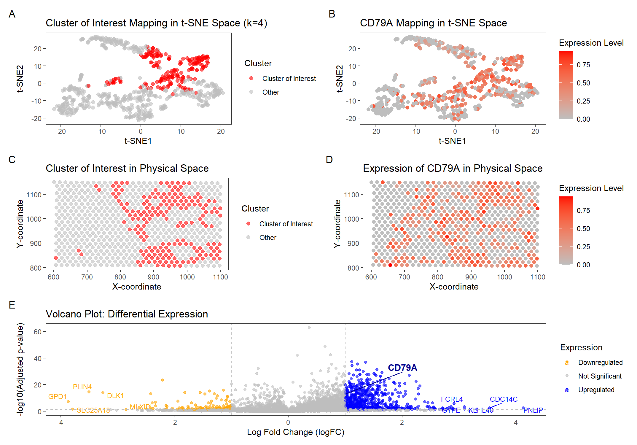
In HW3, I initially selected GJB2 as my gene of interest, assuming it marked an epithelial cell population. However, my differential expression analysis revealed that GJB2 was actually downregulated in the selected cluster, meaning that my original conclusion in HW3—that the cluster represented an epithelial population—was incorrect. Instead, my volcano plot analysis revealed that CD79A, CD19, and MZB1 were the most upregulated genes, all of which are known B cell markers. This suggests that the cluster I originally analyzed in HW3 was actually a B cell population, not an epithelial one. To correct this, I changed my focus to CD79A, allowing me to properly track the same immune cell population between datasets in HW4.

I switched from the Pikachu dataset in HW3 to the Eevee dataset in HW4. The datasets differ significantly in the number of genes and cells – Pikachu has about 17,000 cells and 300 genes, while Eevee has about 700 cells and 18,000 genes. I adjusted my code to change which columns I extracted data from. I also performed k-means clustering with a different k value. In HW3, I used k = 5 in Pikachu. In HW4, for Eevee the elbow plot suggests that using k = 4 is more optimal, based on the total within-cluster sum of squares. This decrease in k makes sense because Eevee (spot-based) has far fewer cells than Pikachu (single-cell resolution), meaning there are naturally fewer distinct groups of cells to separate.

To select the cluster of interest, I computed the mean expression of CD79A across clusters and chose the one with the highest expression. This was Cluster 3, which exhibited significant upregulation of CD79A (logFC = 1.01, adj p-value = 7.75e-14), supporting the hypothesis that this cluster represents a B cell population. In HW3, my B cell cluster also showed strong upregulation of CD19, suggesting that it represents the same immune cell population, so I examined its mean expression in the cluster and confirmed that it is also upregulated. Additionally, one of the top upregulated genes in the cluster was FCRL4, a well-known marker for memory B cells, further reinforcing the presence of B cells in this cluster and aligning with the hypothesis that this cluster corresponds to the same cell type across datasets.

However, some of the other highly upregulated genes in Cluster 3, such as PNLIP (a pancreatic enzyme) and KLHL40 (a muscle-related protein), do not directly align with known B cell markers. This suggests that Cluster 3 may contain a mixed population of cells or activated B cells in a distinct functional state.

Despite this, the combination of CD79A and FCRL4 expression strongly suggests that Cluster 3 contains B cells, potentially memory or regulatory B cells. Comparing this cluster’s transcriptional profile to the Pikachu dataset provides evidence that the same immune cell population is present in both datasets.

Sources

• Morgan, D., & Tergaonkar, V. (2022). Unraveling B cell trajectories at single cell resolution. Trends in Immunology, 43(3), 210–229. https://doi.org/10.1016/j.it.2022.01.003
• Jourdan, M., Robert, N., Cren, M., Thibaut, C., Duperray, C., Kassambara, A., Cogné, M., Tarte, K., Klein, B., & Moreaux, J. (2017). Characterization of human FCRL4-positive B cells. PloS one, 12(6), e0179793. https://doi.org/10.1371/journal.pone.0179793
• National Center for Biotechnology Information (NCBI). (n.d.). PRDM1 PR/SET domain 1 [Homo sapiens (human)]. National Library of Medicine (US),
• National Center for Biotechnology Information. Retrieved [Date of Access], from https://www.ncbi.nlm.nih.gov/gene/5406.
• National Center for Biotechnology Information (NCBI). (n.d.). TCF24 transcription factor 24 [Homo sapiens (human)]. National Library of Medicine (US), National Center for Biotechnology Information. Retrieved [Date of Access], from https://www.ncbi.nlm.nih.gov/gene/131377.

#import libraries
library(ggplot2)
library(patchwork)
library(Rtsne)
library(ggrepel)

set.seed(42)

# Read in data. Cells in rows, genes in columns
data = read.csv("~/Desktop/eevee.csv.gz", row.names = 1)

# Extract data
gexp <- data[,4:ncol(data)]

# Normalize gene expression
gexpnorm <- log10(gexp / rowSums(gexp) * mean(rowSums(gexp)) + 1)


# Examine cell cluster
# pos = data[,2:3]
# df_plot = data.frame(pos, gene = gexpnorm[,'CD79A'])
#
# Plot on tissue to see
# my_color = scale_color_viridis_c(option= "C")
# ggplot(df_plot) + 
#   geom_point(aes(x=aligned_x, y = aligned_y, 
#                  col = gene), size=5) + my_color + 
#   labs(col = "Expression of CD79A", title = "CD79A - Spacial Visualization")+ theme_bw()


# Perform PCA dimensionality reduction
pcs = prcomp(gexpnorm)
plot(pcs$sdev[1:10])

# Perform t-SNE dimensionality reduction 
emb = Rtsne(pcs$x[,1:10])$Y  
df_tsne = data.frame(emb)

#------------------------------------------------------------------------------------------

# Find optimal k using Elbow Method
results <- sapply(2:15, function(i) {
  com <- kmeans(pcs$x[, 1:10], centers = i)
  return(com$tot.withinss)
})
plot(2:15, results, type = "b", xlab = "Number of Clusters (K)", ylab = "Total Within-Cluster Sum of Squares")


# Perform k-means clustering, using a quantitative variable for future changes.
# Based on Elbow plot, use k = 4
k = 4 
com <- as.factor(kmeans(pcs$x[, 1:10], centers = k)$cluster)

df_clusters <- data.frame(tsne_X = emb[,1], tsne_Y = emb[,2], 
                          pca_X = pcs$x[,1], pca_Y = pcs$x[,2], 
                          cluster = com)

ggplot(df_clusters) + geom_point(aes(x = tsne_X, y = tsne_Y, col=cluster), size=3) + theme_bw()


## Cluster Identification

# Compute mean expression of CD79A per cluster
cluster_means <- tapply(gexpnorm[, "CD79A"], com, mean)

# Identify the cluster with the highest CD79A expression using quantitative variable cluster_of_interest
cluster_of_interest <- names(which.max(cluster_means))
print(paste("Cluster with highest CD79A expression:", cluster_of_interest))

# Compute mean expression for other key B cell markers across clusters
b_cell_markers <- c("CD19", "FCRL4")

# Create a data frame to store mean expression of each marker per cluster
cluster_means <- data.frame(cluster = levels(com)) 
for (gene in b_cell_markers) {
  cluster_means[[gene]] <- tapply(gexpnorm[, gene], com, mean, na.rm = TRUE)
}
print(cluster_means)

cluster_means$cluster <- as.character(cluster_means$cluster)

# Identify cluster with highest combined expression for all B cell markers
cluster_highest_b_markers <- cluster_means$cluster[which.max(rowMeans(cluster_means[, b_cell_markers], na.rm = TRUE))]
print(paste("Cluster with highest overall B cell marker expression:", cluster_highest_b_markers))
print(paste("Cluster of Interest:", cluster_of_interest))
# I am using cluster_of_interest <- 3


# Add cluster highlight for visualization
df_clusters$highlight <- ifelse(df_clusters$cluster == cluster_of_interest, "Cluster of Interest", "Other")

# Visualize the cluster of interest in t-SNE space
# ggplot(df_clusters, aes(x = tsne_X, y = tsne_Y, color = highlight)) + 
#   geom_point(alpha = 0.6, size = 2.5) + 
#   theme_minimal() + 
#   scale_color_manual(values = c("red", "grey")) + 
#   labs(title = "Cluster of Interest Highlighted Based on GJB2 Expression",
#        x = "t-SNE1",
#        y = "t-SNE2",
#        color = "Cluster")

# Store 'com' as a factor
df_clusters$cluster <- as.factor(df_clusters$cluster)

# Create a new column to highlight only the selected cluster
df_clusters$highlight <- ifelse(df_clusters$cluster == cluster_of_interest, "Cluster of Interest", "Other")

# Check if 'highlight' column was created correctly
table(df_clusters$highlight)

#------------------------------------------------------------------------------------------

p1 <- ggplot(df_clusters, aes(x = tsne_X, y = tsne_Y, color = highlight)) + 
  geom_point(alpha = 0.6, size = 2) + 
  theme_minimal() + 
  scale_color_manual(values = c("red", "grey")) + 
  labs(title = "Cluster of Interest Mapping in t-SNE Space (k=4)",
       x = "t-SNE1",
       y = "t-SNE2",
       color = "Cluster") +
  theme(plot.title = element_text(size = 7)) + 
  theme(legend.key.size = unit(0.3, "cm")) +
  theme_bw() +
  theme(panel.grid.major = element_blank(), panel.grid.minor = element_blank())

#------------------------------------------------------------------------------------------

# Extract physical coordinates x, y positions
df_clusters$aligned_x <- data[,2]  
df_clusters$aligned_y <- data[,3]  

p2 <- ggplot(df_clusters, aes(x = aligned_x, y = aligned_y, color = highlight)) + 
  geom_point(alpha = 0.6, size = 2) + 
  theme_minimal() + 
  scale_color_manual(values = c("red", "grey")) + 
  labs(title = "Cluster of Interest in Physical Space",
       x = "X-coordinate", 
       y = "Y-coordinate", 
       color = "Cluster") +
  theme(plot.title = element_text(size = 7)) + 
  theme(legend.key.size = unit(0.3, "cm")) +
  theme_bw() +
  theme(panel.grid.major = element_blank(), panel.grid.minor = element_blank())

#------------------------------------------------------------------------------------------

# Compute differential expression for the selected cluster using Wilcox for all genes
pv <- sapply(colnames(gexpnorm), function(i) {
  print(i)
  wilcox.test(gexpnorm[com == cluster_of_interest, i],
              gexpnorm[com != cluster_of_interest, i])$p.val
})

# Compute log2 fold change
logfc <- sapply(colnames(gexpnorm), function(i) {
  print(i)
  log2(mean(gexpnorm[com == cluster_of_interest, i]) /
         mean(gexpnorm[com != cluster_of_interest, i]))
})

#------------------------------------------------------------------------------------------

# Create a dataframe for the Volcano plot
df_volcano <- data.frame(Gene = colnames(gexpnorm), p_value = pv, logFC = logfc)

# Adjust p-values for multiple testing using FDR correction
df_volcano$adj_p_value <- p.adjust(df_volcano$p_value, method = "fdr")

# Convert p-values to -log10 scale for better visualization
df_volcano$logP <- -log10(df_volcano$adj_p_value + 1e-300)

# Define Upregulated and Downregulated Genes
df_volcano$Expression <- "Not Significant"
df_volcano$Expression[df_volcano$logFC > 1 & df_volcano$adj_p_value < 0.05] <- "Upregulated"
df_volcano$Expression[df_volcano$logFC < -1 & df_volcano$adj_p_value < 0.05] <- "Downregulated"

df_volcano <- df_volcano[complete.cases(df_volcano), ]   # Remove rows with NA values
df_volcano <- df_volcano[is.finite(df_volcano$logFC) & is.finite(df_volcano$logP), ]   # Remove Inf values

top_up <- df_volcano[df_volcano$Expression == "Upregulated", ]
if (nrow(top_up) > 5) { top_up <- top_up[order(top_up$logFC, decreasing=TRUE), ][1:5, ] }

top_down <- df_volcano[df_volcano$Expression == "Downregulated", ]
if (nrow(top_down) > 5) { top_down <- top_down[order(top_down$logFC, decreasing=FALSE), ][1:5, ] }

# print(top_up)
# print(top_down)

# Create Volcano Plot
p5 <- ggplot(df_volcano, aes(x = logFC, y = logP, color = Expression)) +
  geom_point(alpha = 0.6) +  
  geom_text_repel(data = top_up, aes(label = Gene), size = 3) +  
  geom_text_repel(data = top_down, aes(label = Gene), size = 3) +
  geom_text_repel(data = df_volcano[df_volcano$Gene == "CD79A", ], 
                  aes(label = Gene), size = 4, color = "darkblue", fontface = "bold", nudge_x=1, nudge_y=20) +
  scale_color_manual(values = c("Upregulated" = "blue", 
                                "Not Significant" = "grey", 
                                "Downregulated" = "orange")) +
  labs(title = "Volcano Plot: Differential Expression",
       x = "Log Fold Change (logFC)",
       y = "-log10(Adjusted p-value)") +
  geom_hline(yintercept = -log10(0.05), linetype = "dashed", color = "grey") +
  geom_vline(xintercept = c(-1, 1), linetype = "dashed", color = "grey") +
  theme(plot.title = element_text(size = 7)) +
  theme_bw() +
  theme(panel.grid.major = element_blank(), panel.grid.minor = element_blank()) 

selected_gene = "CD79A"

# Extract expression of the selected gene from normalized data
df_clusters$gene_expression <- gexpnorm[, selected_gene]

# Observe volcano stats for specific genes
 df_volcano[df_volcano$Gene == selected_gene,]
# df_volcano[df_volcano$Gene == "FCRL4",]
# df_volcano[df_volcano$Gene == "CD19",]


#------------------------------------------------------------------------------------------

# Visualize Gene Expression in t-SNE Space
p3 <- ggplot(df_clusters, aes(x = tsne_X, y = tsne_Y, color = gene_expression)) + 
  geom_point(alpha = 1, size = 2) + 
  theme_minimal() + 
  scale_color_gradient(low="grey", high="red")+ 
  labs(title = paste(selected_gene,"Mapping in t-SNE Space"),
       x = "t-SNE1",
       y = "t-SNE2",
       color = "Expression Level") +
  theme(plot.title = element_text(size = 7)) +
  theme(legend.key.size = unit(0.3, "cm")) +
  theme_bw() +
  theme(panel.grid.major = element_blank(), panel.grid.minor = element_blank()) 

#------------------------------------------------------------------------------------------

p4 <- ggplot(df_clusters, aes(x = aligned_x, y = aligned_y, color = gene_expression)) + 
  geom_point(alpha = 1, size = 2) + 
  theme_minimal() + 
  scale_color_gradient(low="grey", high="red")+
  labs(title = paste("Expression of", selected_gene,"in Physical Space"),
       x = "X-coordinate", 
       y = "Y-coordinate",
       color = "Expression Level") +
  theme(plot.title = element_text(size = 7)) + 
  theme(legend.key.size = unit(0.3, "cm")) +
  theme_bw() +
  theme(panel.grid.major = element_blank(), panel.grid.minor = element_blank())

#------------------------------------------------------------------------------------------

#plots
(p1 + p3) / (p2 + p4) / p5 +
  plot_annotation(tag_levels = 'A')