Multi-Panel Data Visualization of Epithelial Cell Cluster in Eevee Dataset

Hi everyone! My name is Meera Bhat, and I am a BME senior and master's student. I am excited to join this class and learn more about genomic data visualization as I have been working in Dr. Rong Fan's lab at Yale University on spatial omics sequencing and transcriptomics with senescent tissues and would love to learn more. In my free time, I love to read, paint my nails, cook, and dance!

Multi-Panel Data Visualization of Epithelial Cell Cluster in Eevee Dataset

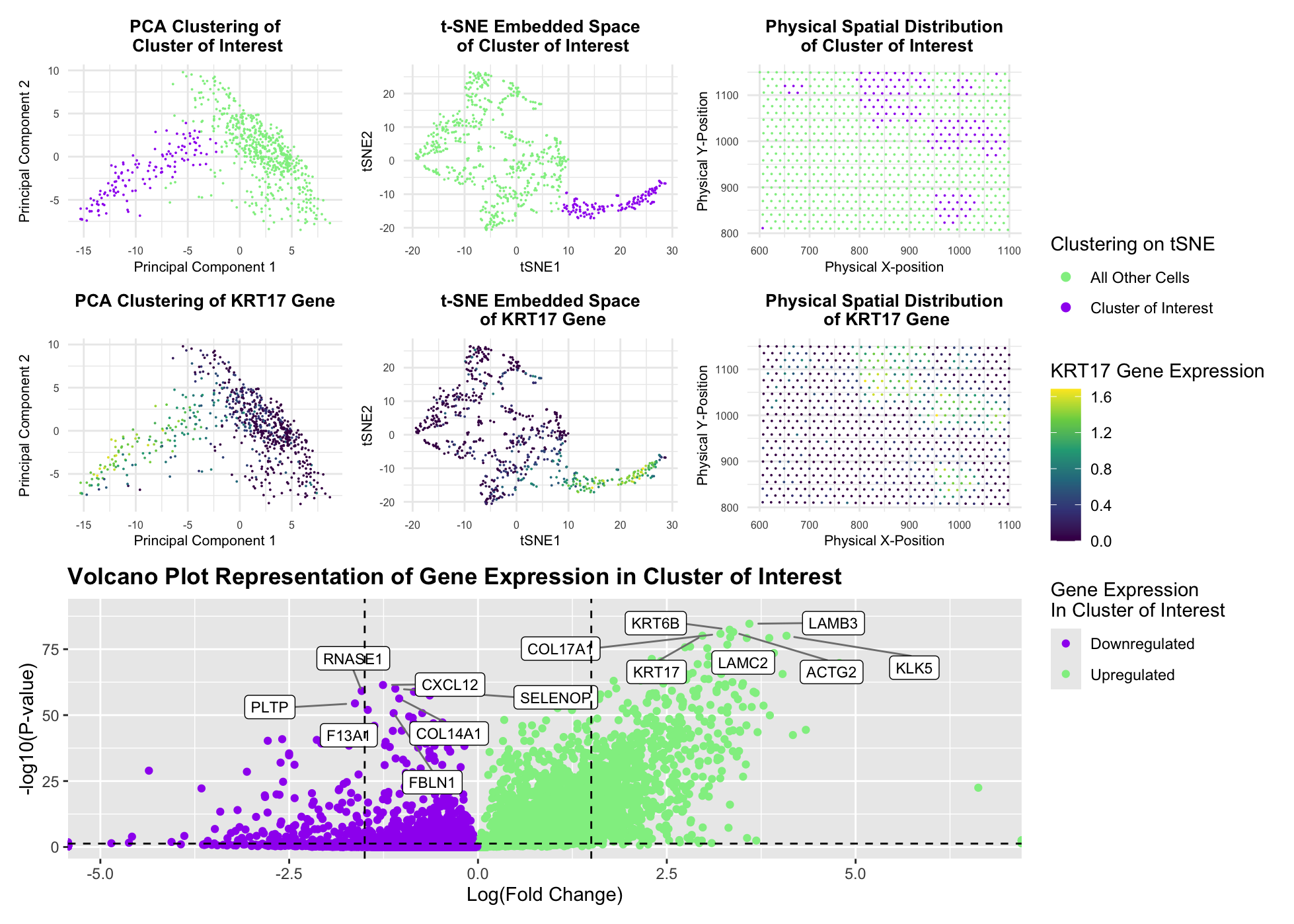
This figure presents an analysis of cellular clusters within the Eevee dataset, focusing on the identification and characterization of a biologically relevant cluster using k-means clustering, dimensionality reduction techniques (PCA and t-SNE), differential gene expression analysis, and statistical analysis through volcano plots. The goal is to determine whether the identified cluster corresponds to the epithelial-like population previously characterized in the Pikachu dataset of HW3, despite differences in the dataset resolution and clustering structure. Principal Component Analysis (PCA) was applied to reduce the dimensionality of the gene expression dataset, improving clustering performance by filtering noise. K-means clustering was then performed on the top principal components to obtain the optimal number of clusters. The top-left PCA plot and top-middle t-SNE plot visualize these clusters, with the cluster of interest highlighted in purple, distinguishing it from the remaining cells (highlighted in green). The top-right physical space plot further confirms that this cluster exhibits a distinct spatial organization within the tissue sample. Furthermore, to identify the optimal PCs needed to account for meaningful variance of the Eevee dataset, visual comparisons were completed to change the number of optimal PCs from 20 in the Pikachu code to 7. In addition to this, the elbow method was additionally utilized to identify the optimal number of clusters (k) for the data. Through identifying the elbow point, the optimal number of clusters was changed from the previous value of 5 to 6. This allowed for the optimal number of clusters for the Eevee dataset. Finally, the presence of the top 2 highly expressed genes from HW3, KRT5 and KRT17, was tested within each cluster of the Eevee dataset to determine that the new cluster of interest would be Cluster 1 (rather than Cluster 2) in order to identify the adequate cell type cluster of epithelial cells with keratinization characteristics.

To assess the biological relevance of this cluster, differentially expressed genes were identified using the Wilcoxon rank-sum test, followed by visualization in the volcano plot (bottom panel). This analysis revealed a set of significantly upregulated genes—KRT17, KRT6B, LAMC2, LAMB3, ACTG2, and KLK5—that distinguish this cluster. Compared to the Pikachu dataset, where epithelial markers such as KRT5, KRT15, KRT16, ELF3, and CEACAM8 were dominant, the Eevee dataset highlights a shift in gene expression patterns, reflecting potential differences in dataset resolution and biological context. However, through further analysis with the Human Protein Atlas, each of these upregulated genes has well-documented associations with epithelial differentiation, extracellular matrix remodeling, and, in some cases, tumorigenesis. KRT17 (Keratin 17), KRT6B (Keratin 6B), LAMC2 (Laminin Subunit Gamma-2), LAMB3 (Laminin Subunit Beta-3), KLK5 (Kallikrein-Related Peptidase 5), and COL17A1 (Collagen type XVII alpha 1 chain) are all shown to exhibit the same squamous epithelial cell line expression that is specific to keratinization, while ACTG2 is found to be expressed in connective tissue cell lines with ECM organization. With this result, it is therefore clear this code identifies the same epithelial cell cluster with tumorigenic characteristics that was previously identified within the Pikachu dataset.

To further confirm the biological identity of the cluster, KRT17 expression levels were mapped in PCA space (middle-left), t-SNE space (middle-center), and physical space (middle-right). The strong enrichment of KRT17 within the cluster supports its epithelial-like properties and potential stress-induced transformation. As well as this, the observed upregulation of basement membrane-associated genes (LAMC2, LAMB3), cytoskeletal regulators (ACTG2), and proteases (KLK5) further indicates a highly dynamic and possibly invasive epithelial population. By adapting the analytical workflow from HW3, I successfully identified an epithelial-like cluster in the Eevee dataset, corresponding to the previously analyzed cluster in the Pikachu dataset. The observed shift from KRT5/KRT15-based markers in Pikachu to KRT17/KRT6B/LAMC2 in Eevee suggests dataset-specific variability with the dramatic increase in genes represented while maintaining epithelial characteristics. The integration of clustering, spatial mapping, and differential gene expression analysis strongly supports the presence of epithelial-enriched features within this cluster. Furthermore, the upregulated genes’ known involvement in tumorigenesis, EMT, and ECM remodeling (validated through HPA and literature sources) provides strong biological justification for the classification of this cluster.

Sources:

Human Protein Atlas: https://www.proteinatlas.org/
https://www.ncbi.nlm.nih.gov/gene/3872
https://www.ncbi.nlm.nih.gov/gene/3854
https://www.ncbi.nlm.nih.gov/gene/3914
https://www.ncbi.nlm.nih.gov/gene/3918
https://www.ncbi.nlm.nih.gov/gene/25818
https://www.ncbi.nlm.nih.gov/gene/72

# Necessary libraries loaded
library(ggplot2)
library(Rtsne)
library(patchwork)
library(dplyr)
library(cluster)
library(factoextra)
library(ggrepel)

# Loads Eevee dataset
file <- '~/Desktop/genomic-data-visualization-2025/data/eevee.csv.gz'
data <- read.csv(file)

# Extracts spatial coordinates and gene expression data from aligned_x and aligned_y columns
pos <- data[, c('aligned_x', 'aligned_y')]
rownames(pos) <- data$cell_id
gexpsub <- data[, 7:ncol(data)]
rownames(gexpsub) <- data$cell_id

# Log-transforms gene expression data and normalizes gexp
normgexpsub <- log10(gexpsub/rowSums(gexpsub) * mean(rowSums(gexpsub)) + 1)

# Performs PCA on gene expression data
pcs <- prcomp(normgexpsub)
plot(pcs$sdev[1:40])

# Finds optimal PCs for kMeans
plot(1:20, pcs$sdev[1:20], type = "l")
plot(1:10, pcs$sdev[1:10], type = "l")

# 7 PCs accounts for meaningful variance of the eevee dataset
pc_opt <- 7

# Perform t-SNE on PCA-reduced gene expression data
set.seed(5)  # Ensures reproducibility

# Determine optimal number of k's (centroids) for kMeans using elbow method
elbow <- fviz_nbclust(normgexpsub, kmeans, method = "wss") +
geom_vline(xintercept = 5, linetype = 2) +
labs(subtitle = "Elbow Method")

elbow

# 6 cluster k's accounts for meaningful variance of the eevee dataset
cluster <- 6

# Perform k-means clustering with k = 6
tsne_emb <- Rtsne(pcs$x[,1:pc_opt])$Y
com <- kmeans(tsne_emb, cluster)

# Creates a data frame for t-SNE visualization
df_tsne <- data.frame(tsne_emb)
colnames(df_tsne) <- c("tSNE1", "tSNE2")
df_tsne$clusters <- as.factor(com$cluster)

# Assigns clusters to data frames
df_clusters <- data.frame(aligned_x = pos$aligned_x, aligned_y = pos$aligned_y,
tSNE1 = tsne_emb[, 1],  tSNE2 = tsne_emb[, 2], kmeans = as.factor(com$cluster))

df_pca <- data.frame(pcs = pcs$x, kmeans = as.factor(com$cluster))
df_pos <- data.frame(pos, clusters = as.factor(com$cluster))

colnames(df_pca)
head(df_pca)
str(df_pca)

# Visualizes the clusters in PC1 vs. PC2 space
pc_cluster <- ggplot(data = df_pca, aes(x = pcs.PC1, y = pcs.PC2, col = cluster)) +
geom_point(size = 1) +
theme_minimal() +
labs(title = "Cell Clusters in PC1 v.s. PC2 Space") +
theme(plot.title = element_text(hjust = 0.5)) +
guides(color = guide_legend(override.aes = list(size = 2.5)))

pc_cluster

# Visualize the clusters in physical space
physical_cluster <- ggplot(data = df_clusters, aes(x = aligned_x, y = aligned_y, col = cluster)) +
geom_point(size = 1) +
theme_minimal() +
labs(title = "Cell Clusters in Physical Space", x = "Aligned X Position", y= "Aligned Y Position") +
theme(plot.title = element_text(hjust = 0.5)) +
guides(color = guide_legend(override.aes = list(size = 2.5)))

physical_cluster

## The top 5 genes identified prior are in prior_gene_list
prior_gene_list <- list("KRT5", "KRT15", "KRT16", "KRT23", "ELF3", "CEACAM8", "PIGR")
for (gene in prior_gene_list) {
# Check if the gene exists as a column name in df_cluster
if (gene %in% colnames(df_clusters)) {
print(gene)
}
}

# Defines a specific gene to visualize (highest expressed gene from hw 3)
selected_gene <- "KRT5"

# Assigns selected gene expression values as numeric value
df_pca$gene <- as.numeric(normgexpsub[, selected_gene])

# Visualizes where KRT5 expression is high
krt5_PCA <- ggplot(data = df_pca, aes(x = pcs.PC1, y = pcs.PC2, col = gene)) +
geom_point(size = 1) +
theme_bw() +
scale_color_gradient(low = 'lightgrey', high = 'blue') +
labs(x = "Principal Component 1", y = "Principal Component 2", color = "KRT5", title = "KRT5 Expression in PCA Space") +
theme(plot.title = element_text(hjust = 0.5))

krt5_PCA

# Defines a specific gene to visualize (second highest expressed gene from hw 3)
selected_gene <- "KRT15"

# Assigns selected gene expression values as numeric value
df_pca$gene <- as.numeric(normgexpsub[, selected_gene])

# Visualizes where KRT15 expression is high
krt15_PCA <- ggplot(data = df_pca, aes(x = pcs.PC1, y = pcs.PC2, col = gene)) +
geom_point(size = 1) +
theme_bw() +
scale_color_gradient(low = 'lightgrey', high = 'blue') +
labs(x = "Aligned X Position", y = "Algned Y Position", color = "KRT15", title = "DSP Expression in PCA Space") +
theme(plot.title = element_text(hjust = 0.5))

krt15_PCA

# Defines cluster of interest
cluster_interest <- 1

# Visualizes cluster of interest, Cluster 1, in PCA space
p1 <- ggplot(df_pca) + geom_point(aes(x = pcs.PC1, y = pcs.PC2,
col = ifelse(kmeans == cluster_interest, "Cluster of Interest", "All Other Cells")),
size = 0.01) +
theme_minimal() +
labs(title = "PCA Clustering of\n Cluster of Interest",
x = "Principal Component 1", y = "Principal Component 2", color = "Clustering on tSNE") +
theme(
plot.title = element_text(size = 10, face = "bold", hjust = 0.5),
axis.title = element_text(size = 8),
axis.text = element_text(size = 6)
) + guides(color = guide_legend(override.aes = list(size = 2)))  +
scale_color_manual(values = c("lightgreen", "purple"))

p1 + krt5_PCA + krt15_PCA # Looks like cluster 1 should be cluster of interest

# Visualizes cluster of interest, Cluster 1, in t-SNE space
p2 <- ggplot(df_clusters) +
geom_point(aes(x = tSNE1, y = tSNE2,
col = ifelse(kmeans == cluster_interest, "Cluster of Interest", "All Other Cells")),
size = 0.01) +
theme_minimal() +
labs(title = "t-SNE Embedded Space\n of Cluster of Interest",
x = "tSNE1", y = "tSNE2", color = "Clustering on tSNE") +
theme(
plot.title = element_text(size = 10, face = "bold", hjust = 0.5),
axis.title = element_text(size = 8),
axis.text = element_text(size = 6)
) + guides(color = guide_legend(override.aes = list(size = 2))) +
scale_color_manual(values = c("lightgreen", "purple"))


# Visualizes cluster of interest, Cluster 1, in physical space
p3 <- ggplot(df_clusters) +
geom_point(aes(x = aligned_x, y = aligned_y,
col = ifelse(kmeans == cluster_interest, "Cluster of Interest", "All Other Cells")),
size = 0.01) +
theme_minimal() +
labs(title = "Physical Spatial Distribution\n of Cluster of Interest",
x = "Physical X-position", y = "Physical Y-Position", color = "Clustering on tSNE") +
theme(
plot.title = element_text(size = 10, face = "bold", hjust = 0.5),
axis.title = element_text(size = 8),
axis.text = element_text(size = 6)
) + guides(color = guide_legend(override.aes = list(size = 2)))  +
scale_color_manual(values = c("lightgreen", "purple"))

# Visualizes differentially expressed genes for cluster of interest, Cluster 1
com_categories = as.factor(com$cluster)
p_value = sapply(colnames(normgexpsub), function(i){
print(i)
wilcox.test(normgexpsub[com_categories == cluster_interest, i], normgexpsub[com_categories!= cluster_interest, i])$p.val
})

logfc = sapply(colnames(normgexpsub), function(i){
print(i)
log2(mean(normgexpsub[com_categories == cluster_interest, i])/mean(normgexpsub[com_categories != cluster_interest, i]))
})


# Creates a volcano plot dataframe
df_volcano <- data.frame(
p_value = -log10(p_value + 1e-100),
logfc,
genes = colnames(normgexpsub)
)

# Removes NA values from df_volcano to reduce warning message error
df_volcano <- df_volcano[complete.cases(df_volcano), ]

# Adjusts threshold for gene labeling to avoid excessive overlap of labels
df_volcano$gene_label <- ifelse(
df_volcano$p_value > 10 & abs(df_volcano$logfc) > 1.5,
as.character(df_volcano$genes),
NA
)

#Assigns number of labels as 7 to allow for proper labeling without excessive overlap
num_labels_down <- 7
num_labels_up <- 7

top_down <- df_volcano %>% filter(logfc < -1) %>% top_n(num_labels_down, wt = p_value)
top_up <- df_volcano %>% filter(logfc > 1) %>% top_n(num_labels_up, wt = p_value)

df_volcano$gene_label <- ifelse(
df_volcano$genes %in% c(top_down$genes, top_up$genes),
as.character(df_volcano$genes),
NA
)

# Generates volcano plot
volcano_plot <- ggplot(df_volcano) +
geom_point(aes(x = logfc, y = p_value, col = ifelse(logfc > 0, 'Upregulated', 'Downregulated'))) +
geom_label_repel(aes(x = logfc, y = p_value, label = gene_label), box.padding = 0.5,
point.padding = 0.5, segment.color = 'grey50', max.overlaps = 30, min.segment.length = 0.5,
force = 2, size = 3) +
ylim(0, max(df_volcano$p_value) + 5) + geom_hline(yintercept = -log10(0.05), linetype = "dashed") +
geom_vline(xintercept = c(-1.5, 1.5), linetype = "dashed") +
labs(col = "Gene Expression\nIn Cluster of Interest",
title = "Volcano Plot Representation of Gene Expression in Cluster of Interest",
x = "Log(Fold Change)", y = "-log10(P-value)") +
theme(plot.title = element_text(face = "bold")) +
scale_color_manual(values = c("purple", "lightgreen"))

# Displays the volcano plot to identify clusters of downregulated and upregulated genes
volcano_plot

# Defines a specific gene to visualize
selected_gene <- "KRT17"

# Assigns selected gene expression values as numeric value
df_pca$gene <- as.numeric(normgexpsub[, selected_gene])
df_tsne$gene <- as.numeric(normgexpsub[, selected_gene])
df_pos$gene <- as.numeric(normgexpsub[, selected_gene])

# Visualizes selected gene in PCA space
p4 <- ggplot(df_pca, aes(x = pcs.PC1, y = pcs.PC2, col = gene)) +
geom_point(size = 0.01) +
scale_color_viridis_c() +
theme_minimal() +
labs(title = "PCA Clustering of KRT17 Gene",
x = "Principal Component 1", y = "Principal Component 2", color = "KRT17 Gene Expression") +
theme(
plot.title = element_text(size = 10, face = "bold", hjust = 0.5),
axis.title = element_text(size = 8),
axis.text = element_text(size = 6)
)

# Visualizes selected gene in t-SNE space
df_tsne$gene <- normgexpsub[, selected_gene]
p5 <- ggplot(df_tsne, aes(x = tSNE1, y = tSNE2, col = gene)) +
geom_point(size = 0.01) +
scale_color_viridis_c() +
theme_minimal() +
labs(title = "t-SNE Embedded Space\n of KRT17 Gene",
x = "tSNE1", y = "tSNE2", color = "KRT17 Gene Expression") +
theme(
plot.title = element_text(size = 10, face = "bold", hjust = 0.5),
axis.title = element_text(size = 8),
axis.text = element_text(size = 6)
)

# Visualizes selected gene in physical space
df_pos$gene <- normgexpsub[, selected_gene]
p6 <- ggplot(df_pos, aes(x = aligned_x, y = aligned_y, col = gene)) +
geom_point(size = 0.01) +
scale_color_viridis_c() +
theme_minimal() +
labs(title = "Physical Spatial Distribution\n of KRT17 Gene",
x = "Physical X-Position", y = "Physical Y-Position", color = "KRT17 Gene Expression") +
theme(
plot.title = element_text(size = 10, face = "bold", hjust = 0.5),
axis.title = element_text(size = 8),
axis.text = element_text(size = 6)
)

# Combines all plots together for visualization
(p1 + p2 + p3) / (p4 + p5 + p6) / volcano_plot +
plot_layout(heights = c(1, 1, 1.5), guides = "collect")


# Sources:
# https://www.datacamp.com/doc/r/cluster
# https://rpkgs.datanovia.com/factoextra/
# https://ggrepel.slowkow.com/
# code-lesson-5.R
# code-lesson-6.R
# code-lesson-7.R
# code-lesson-8.R
# https://www.statology.org/set-seed-in-r/
# https://www.appsilon.com/post/r-tsne
# https://www.datacamp.com/tutorial/pca-analysis-r
# https://www.datacamp.com/tutorial/k-means-clustering-r
# https://www.rdocumentation.org/packages/base/versions/3.6.2/topics/data.frame
# https://stackoverflow.com/questions/21271449/how-to-apply-the-wilcox-test-to-a-whole-dataframe-in-r
# https://biostatsquid.com/volcano-plots-r-tutorial/
# https://www.geeksforgeeks.org/how-to-create-and-visualise-volcano-plot-in-r/
# https://sjmgarnier.github.io/viridis/reference/scale_viridis.html
# https://www.analyticsvidhya.com/blog/2021/01/in-depth-intuition-of-k-means-clustering-algorithm-in-machine-learning/
# https://www.rdocumentation.org/packages/patchwork/versions/1.3.0/topics/plot_layout

19 Feb 2025

« Identification of Adipocyte-like/Lipid-metabolizing Cells in Breast Cancer Tissue Multi-dimensional Analysis of HER2+ Cells: Spatial Distribution and Gene Expression Patterns »