Analysis of Sequencing Data Cluster 7 and AGR3 Expression

1.
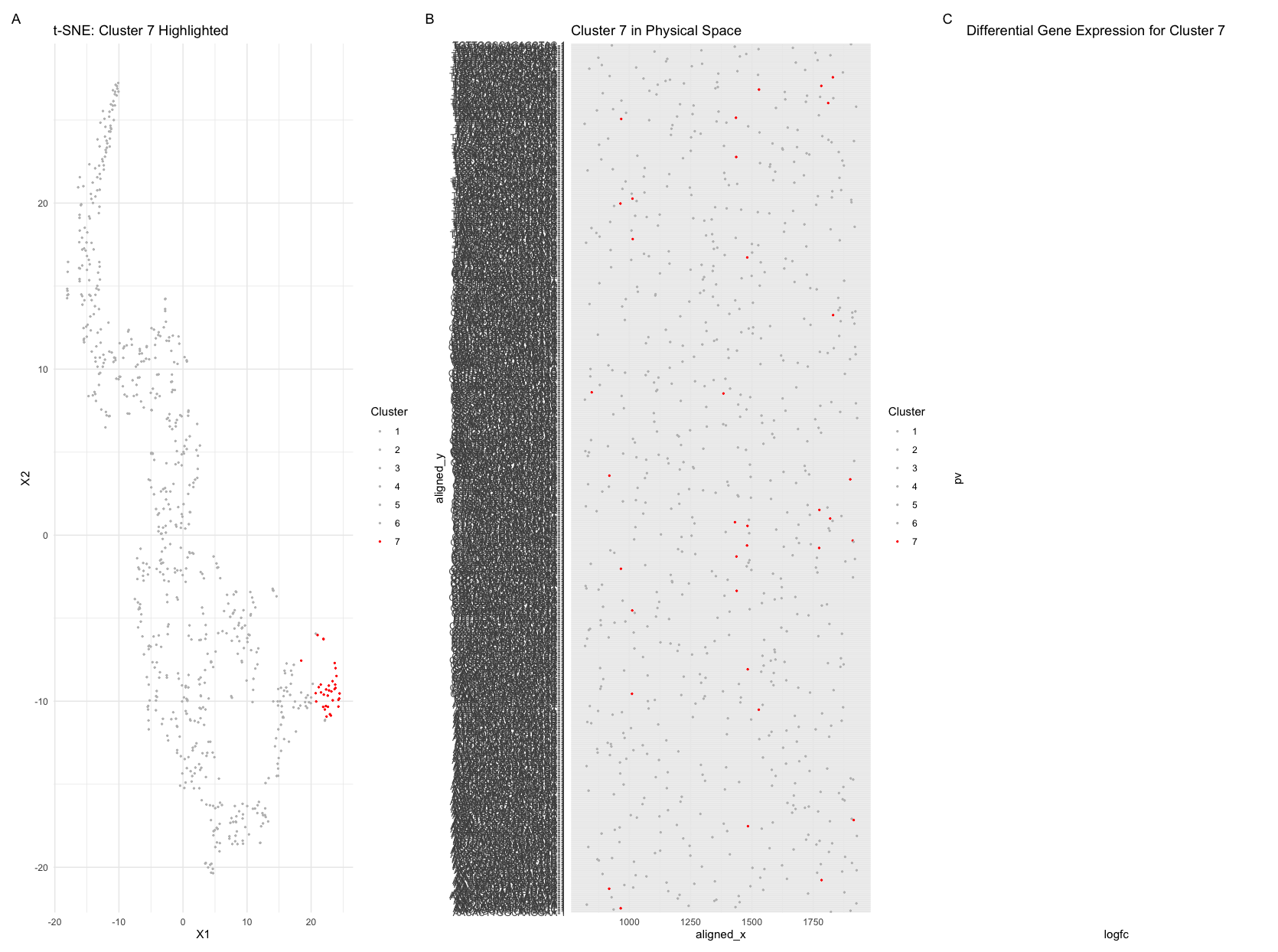
Because I could not find the cluster I had identified in HW 3, I decided to restart and look at a different cluster and gene (highest expression). Since I had been using Pikachu, I switched to Eevee for this homework. I found that with the new dataset, it took much fewer PCs after PCA with the new dataset and the variation was still captured. The Pikachu dataset was an imaging dataset, so there was more variation than the Eevee dataset that is sequencing based. From my redo of HW 3, I had fewer clusters in the Eevee dataset analysis (I had 7 clusters) and chose to analyze cluster 7. To find the same cluster I identified on the Pikachu dataset, I looked for a high expression of the same gene (AGR3) and found where the highest expressions were in cluster 7. I found that it was the same spatial orientation and the cells still had the highest AGR3 expression. Between the redone HW 3 assignment and this HW on Eevee, I think the cells of interest were still the same groupings as the imaging dataset based on location. The cells are tightly grouped together, which also aligns with being a cancer cell. With this, I think the identified cells are the same across the two datasets.
2. Code (paste your code in between the ``` symbols)
1
2
3
4
5
6
7
8
9
10
11
12
13
14
15
16
17
18
19
20
21
22
23
24
25
26
27
28
29
30
31
32
33
34
35
36
37
38
39
40
41
42
43
44
45
46
47
48
49
50
51
52
53
54
55
56
57
58
59
60
61
62
63
64
65
66
67
68
69
70
71
72
73
74
75
76
77
78
79
80
81
82
83
84
85
86
87
88
89
# Load necessary libraries
library(ggplot2)
library(Rtsne)
library(patchwork)

# Read and preprocess data
file_path <- '~/Desktop/genomic-data-visualization-2025/data/eevee.csv.gz'
dataset <- read.csv(file_path)

# Extract spatial coordinates and gene expression values
coordinates <- dataset[, 1:2]
names(coordinates) <- c("aligned_x", "aligned_y")  # Ensure column names are consistent
gene_data <- dataset[, 3:ncol(dataset)]

# Normalize gene expression data
normalized_gene_data <- log10((gene_data + 1) / rowSums(gene_data + 1) * mean(rowSums(gene_data + 1)))

# Perform PCA for dimensionality reduction
pca_result <- prcomp(normalized_gene_data, center = TRUE, scale. = TRUE)
embedding <- Rtsne(pca_result$x[, 1:9], perplexity = 30, max_iter = 500)$Y

# Apply k-means clustering with 7 centers
set.seed(123)
cluster_assignment <- kmeans(normalized_gene_data, centers = 7, nstart = 10)$cluster
cluster_assignment <- as.factor(cluster_assignment)

# Identify differentially expressed genes efficiently
calculate_top_gene <- function(cluster) {
  p_values <- sapply(colnames(normalized_gene_data), function(gene) {
    tryCatch(
      wilcox.test(normalized_gene_data[cluster_assignment == cluster, gene],
                  normalized_gene_data[cluster_assignment != cluster, gene])$p.value,
      error = function(e) NA
    )
  })
  p_values <- na.omit(p_values)
  if (length(p_values) > 0) {
    return(names(sort(p_values, decreasing = FALSE)[1]))
  } else {
    return(NA)
  }
}

top_genes <- sapply(1:7, calculate_top_gene)

# Target gene analysis
target_gene <- top_genes[7]
if (!is.na(target_gene)) {
  expression_cluster7 <- normalized_gene_data[cluster_assignment == 7, target_gene]
  expression_other <- normalized_gene_data[cluster_assignment != 7, target_gene]

  if (all(expression_cluster7 > 0) & all(expression_other > 0)) {
    t_test_result <- t.test(expression_cluster7, expression_other)$p.value
    log_fc <- log2(mean(expression_cluster7) / mean(expression_other))
  } else {
    t_test_result <- NA
    log_fc <- NA
  }
} else {
  t_test_result <- NA
  log_fc <- NA
}

# Ensure valid numerical values for volcano plot
if (!is.na(t_test_result) && !is.na(log_fc)) {
  volcano_data <- data.frame(pv = -log10(t_test_result), logfc = log_fc)
} else {
  volcano_data <- data.frame(pv = numeric(0), logfc = numeric(0))
}

# Visualization
plot_tsne <- ggplot(data.frame(embedding, Cluster = cluster_assignment)) +
  geom_point(aes(x = X1, y = X2, col = Cluster), size = 0.4) +
  scale_color_manual(values = c(rep("gray", 6), "red")) +
  labs(title = "t-SNE: Cluster 7 Highlighted") + theme_minimal()

plot_physical <- ggplot(data.frame(coordinates, Cluster = cluster_assignment)) +
  geom_point(aes(x = aligned_x, y = aligned_y, col = Cluster), size = 0.4) +
  scale_color_manual(values = c(rep("gray", 6), "red")) +
  labs(title = "Cluster 7 in Physical Space") + theme_minimal()

volcano_plot <- ggplot(volcano_data) +
  geom_point(aes(x = logfc, y = pv), color = "blue") +
  labs(title = "Differential Gene Expression for Cluster 7") + theme_minimal()

final_plot <- plot_tsne + plot_physical + volcano_plot + plot_annotation(tag_levels = 'A')

ggsave("~/Desktop/Genomic Data Visualization Code/hw4_newimage.png", final_plot, width = 16.70, height = 12.44, units = "in", dpi = 100)