Description

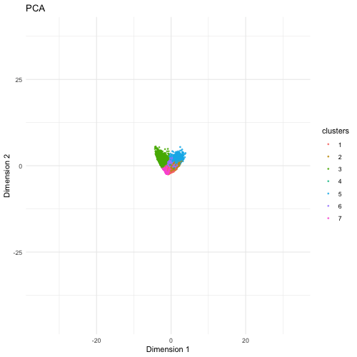
The visualization compares three different dimensionality reduction techniques—PCA (Principal Component Analysis), t-SNE (t-Distributed Stochastic Neighbor Embedding), and UMAP (Uniform Manifold Approximation and Projection)—to visualize high-dimensional gene expression data from Pikachu dataset in 2D. PCA is a linear method that projects data onto the directions of highest variance. It preserves the global structure but sometimes fails to capture nonlinear relationships in complex datasets. It provides a quick overview but may not separate cell types well. t-SNE is a nonlinear method that better captures local relationships by clustering similar cells together, but distances between clusters may not always be meaningful. If the focus is on local relationships and identifying distinct cell populations, t-SNE and UMAP would be better. UMAP is another nonlinear technique that preserves both local and some global structure, often producing well-separated clusters that reflect biological heterogeneity.

library(ggplot2)
library(gganimate)
library(Rtsne)
library(umap)
library(tidyverse)
# Load the dataset
data <- read.csv("./data/pikachu.csv.gz")
pos <- data[, 5:6]
rownames(pos) <- data$cell_id
gexp <- data[, 7:ncol(data)]
rownames(gexp) <- data$barcode
loggexp <- log10(gexp+1)
com <- kmeans(loggexp, centers=7)
clusters <- com$cluster
clusters <- as.factor(clusters) 
names(clusters) <- rownames(gexp)
pcs <- prcomp(loggexp)
emb_pca <- pcs$x[, 1:2]
emb_tsne <- Rtsne::Rtsne(loggexp)$Y
emb_umap <- umap::umap(loggexp)$layout
## Combine results 
df_pca <- data.frame(emb_pca, clusters, method = "PCA")
df_tsne <- data.frame(emb_tsne, clusters, method = "t-SNE")
df_umap <- data.frame(emb_umap, clusters, method = "UMAP")
colnames(df_pca) <- colnames(df_tsne) <- colnames(df_umap) <- c('x', 'y', 'clusters', 'method')
df_combined <- rbind(df_pca, df_tsne, df_umap)
ggplot(df_combined, aes(x=x, y=y, col=clusters)) + 
  geom_point(size=0.5, alpha=0.7) +
  facet_wrap(~method) +
  labs(title = "Comparison of Dimensionality Reduction Methods", x = "Dimension 1", y = "Dimension 2") +
  theme_minimal()
p <- ggplot(df_combined, aes(x=x, y=y, col=clusters)) +
  geom_point(size = 0.5, alpha=0.7) +
  theme_minimal() +
  labs(title = "{closest_state}", x = "Dimension 1", y = "Dimension 2") +
  transition_states(method, transition_length = 2, state_length = 1)
anim <- animate(p, height=500, width=500, renderer = gifski_renderer())
anim_save("dim_reduction_comparison.gif", animation = anim)