Interrogating Cell Type with CODEX Spleen Dataset

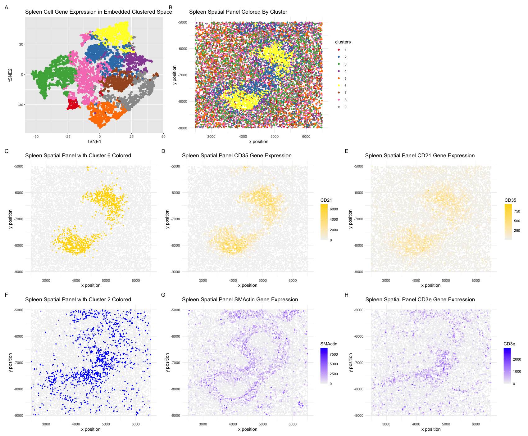
I select clusters 6 and 2 for further analysis given their distinctive spatial organization. Performing differential gene expression analysis on cluster 6 with the Wilcox “greater-than” test yields significant gene hits led by CD20, CD21, CD35, and CD44. Performing the same differential gene expression analysis statistical testing on cluster 2 reveals prolific upregulation of SMactin, CD45, CD3e, and CD4. Visualizing these top hits – CD20 and CD35 for cluster 6, SMactin and CD25 for cluster 6– reveals strong spatial correlation with their respective associated clusters. CD20, for example, is heavily expressed in the cluster 6 cells relative to surrounding cells, while SMactin is selectively expressed primarily in cluster 2.
CD20 is a prolific B-lymphocyte marker, starting from late pro-B lymphocytes. It is known to be expressed in the splennic white pump, particularly in the follicles and marginal zones. CD35, on the other hand, is heavily implicated in the follicular dendritic cell-mediated presentation of antigen-antibody immune complexes to B cells during the secondary immune response. Cluster 6, is highly likely to comprise primarily B cells, with some follicular dendritic cell character (CD35) not unexpected given the phenotypic and spatial complexity of the mechanism of B-lymphocyte activation.
In cluster 2: SMactin is known as an indicator of inflammatory pseudotumors (IPTs), particularly in differentiating with IPT-like FDC sarcomas. It has also been noted to be positive in splenic parenchymal myofibroblasts, particularly found adjacent to white and red pulp in disordered conditions. Meanwhile, CD3e is a known T-cell marker, expressed in almost all T-cell lymphomas and leukemias. The protein encoded by CD3e is expressed in the cytoplasm and acts as an immune recognition receptor. Cluster 2 likely comprises a more prominant myofibroblast presence with some T-cell character, likely characterizing the periarteriolar lymphoid sheath (PALS, T-cell presence) in the white pulp.
I therefore conclude that the CODEX spleen dataset primarily depicts the white pulp of the spleen–particularly in the selected clusters–, rich with B cells and adjacent myofibroblasts and associated T-cells. Potent gene expression markers of these immune types dominate the dataset, while the morphology is also suggestive of the characteristic marginal zone (B-cell area), adjacent follicles (B-cells), and periarteriolar lymphoid sheath (T-cell) surround a central arteriole; this would facilitate lymphoid transport and interaction with the described B cells and T cells, as well as structural elements.
- https://meridian.allenpress.com/aplm/article/143/9/1093/421104/Practical-Applications-in-Immunohistochemistry-An
- https://academic.oup.com/intimm/article-abstract/16/1/119/721734?redirectedFrom=PDF
- https://pmc.ncbi.nlm.nih.gov/articles/PMC1939903/
- https://pmc.ncbi.nlm.nih.gov/articles/PMC4508554/#:~:text=IPT
- https://www.ncbi.nlm.nih.gov/gene/916
- https://www.neobiotechnologies.com/product/cd3e-t-cell-marker-2/?srsltid=AfmBOorf0pZwfs5JBWLj_oQEYB4HFsCjMHdT464V4HvKZQoJPcx3fX7d
- https://pmc.ncbi.nlm.nih.gov/articles/PMC1828535/
5. Code (paste your code in between the ``` symbols)
1
2
3
4
5
6
7
8
9
10
11
12
13
14
15
16
17
18
19
20
21
22
23
24
25
26
27
28
29
30
31
32
33
34
35
36
37
38
39
40
41
42
43
44
45
46
47
48
49
50
51
52
53
54
55
56
57
58
59
60
61
62
63
64
65
66
67
68
69
70
71
72
73
74
75
76
77
78
79
80
81
82
83
84
85
86
87
88
89
90
91
92
93
94
95
96
97
98
99
100
101
102
103
104
105
106
107
108
109
110
111
112
113
114
115
116
117
118
119
120
121
122
123
124
125
126
127
128
129
130
131
132
133
134
135
136
137
138
139
140
141
142
143
144
145
146
147
148
149
150
151
152
153
154
155
156
157
158
159
160
161
162
163
164
165
166
167
168
169
170
171
172
173
174
175
176
177
178
179
180
181
182
183
184
185
186
187
188
189
190
191
192
193


library(ggplot2)
library(patchwork)
library(Rtsne)
library(ggrepel)

data <- read.csv('codex_spleen_3.csv.gz')

data[1:5,1:5]


## 10,000 cells, 28 genes --> CODEX spleen set.

pos <- data[,2:4]
gexp <- data[, 5:ncol(data)]
head(pos)
head(gexp)
dim(gexp)
norm <- gexp/rowSums(gexp) * 10000
rowSums(norm)


# dimensional embedding/clustering


## determine optimal cluster quantity

#elbow <- sapply(2:20, function(k) {
#  out <- kmeans(norm, centers = k)
#  out$tot.withinss
#})

#plot(2:20, elbow)

#elbow <- data.frame(x = 2:20, y = elbow)
#ggplot(elbow, aes(x=x, y=y, col = 'red', size = 0.5)) +
#  geom_point() +
#  xlab("Cluster Quantity") +
#  ylab("Total Withiness") +
#  theme(legend.position = "none") +
#  scale_size(range = c(2,2))


com <- kmeans(norm, centers = 9)
clusters <- com$cluster
head(clusters)
pos['clusters'] = clusters
pos$clusters <- factor(cut(pos$clusters, breaks = 9))


## visualize spatial distribution of cells and areas
g2<- ggplot(pos, aes(x=x, y=y, size = sqrt(area), col = clusters)) +
  geom_point() +
  scale_size(range = c(0.5,1.5)) +  # Adjust range for smaller points
  theme_minimal() +
  guides(size = "none") +
  scale_color_brewer(palette = "Set1", labels = c("1", "2", "3", "4", "5", "6", "7", "8", "9")) +
  xlab("x position") +
  ylab("y position") +
  ggtitle('Spleen Spatial Panel Colored By Cluster')

emb <- Rtsne::Rtsne(norm)
df <- data.frame(emb$Y, clusters)
g1 <- ggplot(df, aes(x = X1, y = X2, col=pos$clusters)) +
  geom_point() +
  scale_color_brewer(palette = "Set1", labels = c("1", "2", "3", "4", "5", "6", "7", "8", "9")) +
  xlab("tSNE1") +
  ylab("tSNE2") +
  theme(legend.position = "none") +
  ggtitle('Spleen Cell Gene Expression in Embedded Clustered Space')


## Interrogate cluster 6

pos$cluster_6 <- ifelse(df$clusters == 6, "Cluster 6", "Other")
g3 <- ggplot(pos, aes(x = x, y = y, size = sqrt(area), col = cluster_6)) +
  geom_point() +
  scale_color_manual(values = c("Cluster 6" = "#FFD700", "Other" = "#F2F2F2")) +
  labs(color = "Cluster 6") +
  scale_size(range = c(0.5, 1.0)) +
  theme_minimal() +
  ggtitle('Spleen Spatial Panel with Cluster 6 Colored') +
  xlab("x position") +
  ylab("y position") +
  guides(size = "none") +
  theme(legend.position = "none")


g5 <- ggplot(pos, aes(x = x, y = y,size = sqrt(area), col = norm[,'CD35'])) +
  geom_point() +
  scale_color_gradient(high = "#FFD700", low = "#F2F2F2") +
  labs(color = 'CD35') +
  scale_size(range = c(0.5, 1.0)) +
  #labs(color = "Cluster 1") +
  theme_minimal() +
  ggtitle('Spleen Spatial Panel CD21 Gene Expression') +
  xlab("x position") +
  guides(size = "none") +
  ylab("y position")
  #theme(legend.position = "none")

g7 <- ggplot(pos, aes(x = x, y = y,size = sqrt(area), col = norm[,'CD21'])) +
  geom_point() +
  scale_color_gradient(high = "#FFD700", low = "#F2F2F2") +
  labs(color = 'CD21') +
  scale_size(range = c(0.5, 1.0)) +
  #labs(color = "Cluster 1") +
  theme_minimal() +
  ggtitle('Spleen Spatial Panel CD35 Gene Expression') +
  xlab("x position") +
  guides(size = "none") +
  ylab("y position")
#theme(legend.position = "none")


norm['clusters'] = clusters
gexp['clusters'] = clusters
ct1 <- which(clusters == 6)
ctother <- which(clusters != 6)
results_6 <- sapply(colnames(norm), function(i) {
  wilcox.test(norm[ct1, i], norm[ctother, i], alternative = 'greater')$p.value
})
#name(results_1) <- colnames(norm)
sort(results_6[results_6 < 0.05])

# greatest hits: CD20, CD21, CD35. CD44. HLA.DR, CD1c


## Interrogate cluster 2
pos$cluster_2 <- ifelse(df$clusters == 2, "Cluster 2", "Other")
g4 <- ggplot(pos, aes(x = x, y = y,size = sqrt(area), col = cluster_2)) +
  geom_point() +
  scale_color_manual(values = c("Cluster 2" = "blue", "Other" = "#F2F2F2")) +
  labs(color = "Cluster 2") +
  scale_size(range = c(0.5, 1.0)) +
  theme_minimal() +
  ggtitle('Spleen Spatial Panel with Cluster 2 Colored') +
  xlab("x position") +
  ylab("y position") +
  guides(size = "none") +
  theme(legend.position = "none")


g6 <- ggplot(pos, aes(x = x, y = y,size = sqrt(area), col = norm[,'SMActin'])) +
  geom_point() +
  scale_color_gradient(high = "blue", low = "#F2F2F2") +
  labs(color = 'SMActin') +
  scale_size(range = c(0.5, 1.0)) +
  #labs(color = "Cluster 1") +
  theme_minimal() +
  ggtitle('Spleen Spatial Panel SMActin Gene Expression') +
  xlab("x position") +
  guides(size = "none") +
  ylab("y position")
#theme(legend.position = "none")

g8 <- ggplot(pos, aes(x = x, y = y,size = sqrt(area), col = norm[,'CD3e'])) +
  geom_point() +
  scale_color_gradient(high = "blue", low = "#F2F2F2") +
  labs(color = 'CD3e') +
  scale_size(range = c(0.5, 1.0)) +
  #labs(color = "Cluster 1") +
  theme_minimal() +
  ggtitle('Spleen Spatial Panel CD3e Gene Expression') +
  xlab("x position") +
  guides(size = "none") +
  ylab("y position")
#theme(legend.position = "none")

ct1 <- which(clusters == 2)
ctother <- which(clusters != 2)
results_2 <- sapply(colnames(norm), function(i) {
  wilcox.test(norm[ct1, i], norm[ctother, i], alternative = 'greater')$p.value
})
#name(results_1) <- colnames(norm)
sort(results_2[results_2 < 0.05])


# top hits: SMActin, CD20, CD45


(g1 + g2 + plot_spacer()) / (g3 + g7 + g5) / (g4 + g6 + g8) + plot_annotation(tag_levels = 'A')


###