Uncovering spleen tissue type

[description]

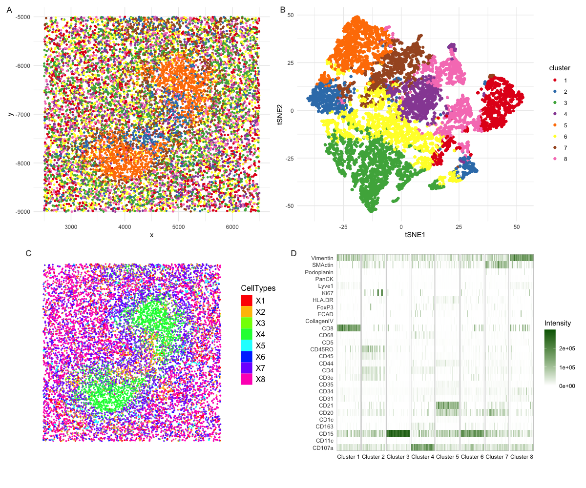
1. Figure caption Figure A and B share the same legend. Figure A shows the physical location of each cell on this tissue slide and each cell is colored by the cluster assignment created from Kmean clustering (k=8). Figure B is tSNE plot where each dot is a cell colored with the same color scheme. Figure C is generated from R package STdeconcolve. Each dot is a pie chart colored by the cell type. Figure D is a heatmap for all the proteins included in the dataset. X axis is ordered by cluster assignment created by the same Kmean clustering, and each vertical line represent one cell in a cluster. The color represents the intensity associated with the protein in the cell.

2. What type of spleen tissue? White pulp

3. Why this conclusion? Figure A reveals unique structure of the tissue slide where most of the clusters are mixed in the physical space but cluster 5 (orange). Figure B also shows that cluster 5 forms a distinct cluster itself. This cluster of cells are validated by figure C, however, the cells are less mixed in the physical space. Moreover, figure C shows that the cell cluster is enclosed by another cell type, and figure A vaguely reveals similar patterns. In figure D, we can look at the protein composition in each cell cluster. Cluster 5 mainly expresses CD21 and CD20 which are markers for B cells and cluster 7 mainly express SMActin which can be found in smooth muscle cells in blood vessels (1). When looking at other clusters that are mixed in the physical space, we see most of them express Vimentin which could help lymphocytes migrate and home to spleen (2). They also express different combinations of CD proteins representing various immune cells. Based on evidences above and the comparison to histology slides (3,4), it is highly likely this tissue is the white pulp from spleen.

Reference

1. https://pmc.ncbi.nlm.nih.gov/articles/PMC6205219/
2. https://www.nature.com/articles/ncb1355
3. https://vmicro.iusm.iu.edu/hs_vm/docs/lab7_6.htm
4. https://storymd.com/journal/qjorvlxtnj-spleen/page/knlklh93dg-spleen

library(tidyverse)
library(ggplot2)
library(patchwork)

codex <- read.csv("~/Documents/genom_visual/hw5/codex_spleen_3.csv")

pos=codex[,2:3]
rownames(pos) <- codex$X
exp=log10(codex[,5:32]/rowSums(codex[,5:32])+1)*1e6
rownames(exp) <- codex$X

set.seed(66)
# tw = sapply(2:15, function(x) kmeans(exp, centers=x)$tot.withinss)
# plot(2:15, tw)

km = kmeans(exp, centers=8)
clusters <- as.factor(km$cluster)
names(clusters) <- rownames(exp)

df = cbind(pos, clusters)
p1=ggplot(df, aes(x=x, y=y, colour=clusters)) + 
  geom_point(size=1)+
  scale_color_brewer(palette = "Set1")+
  theme_minimal()+
  theme(legend.position = "none")


tsne <- Rtsne::Rtsne(exp)
df= as.data.frame(tsne$Y)%>% mutate(cluster=clusters, tSNE1=V1, tSNE2=V2)
p2=ggplot(df, aes(x=tSNE1, y=tSNE2, colour=cluster)) + 
  geom_point()+
  scale_color_brewer(palette = "Set1")+
  theme_minimal()


library(STdeconvolve)
## remove pixels with too few genes
counts <- cleanCounts(t(round(exp)), min.lib.size = 10)
## feature select for genes
corpus <- restrictCorpus(counts, removeAbove=1.0, removeBelow = 0.05)
## choose optimal number of cell-types
ldas <- fitLDA(t(as.matrix(corpus)), Ks = c(4,6,7,8,9,10))
## get best model results
optLDA <- optimalModel(models = ldas, opt = "min")
## extract deconvolved cell-type proportions (theta) and transcriptional profiles (beta)
results <- getBetaTheta(optLDA, perc.filt = 0.05, betaScale = 1000)
deconProp <- results$theta
deconGexp <- results$beta
## visualize deconvolved cell-type proportions
p3=vizAllTopics(deconProp, pos,r=20, lwd=0)


df=cbind(clusters,exp)%>%
  #select(clusters, CD4,CD8,CD20,CD45,SMActin,ECAD,FoxP3,Ki67,Podoplanin)%>%
  arrange(clusters)%>%
  group_by(clusters)%>%
  mutate(ID=row_number(),
         clust=paste0("Cluster ", clusters)) %>%
  ungroup()%>%
  pivot_longer(names_to = "protein", values_to = "intensity", cols = 2:29)

p4=ggplot(df, aes(x=ID, y=protein, fill=intensity))+
  geom_tile()+
  facet_grid(.~clust, scales = "free_x",switch = "x")+
  scale_fill_gradient(low="white", high="darkgreen", name="Intensity")+
  scale_x_discrete(drop = TRUE)+
  scale_y_discrete(expand = c(0, 0)) +
  xlab("")+
  ylab("")+
  theme_minimal()+
  theme(panel.spacing = unit(0.05, "cm"),
        strip.switch.pad.grid = unit(0, "cm"),
        panel.border = element_rect(color = "grey", fill = NA, linewidth = 0.5))

(p1 + p2) / (p3 + p4) + plot_layout(widths = c(1, 1))