Description

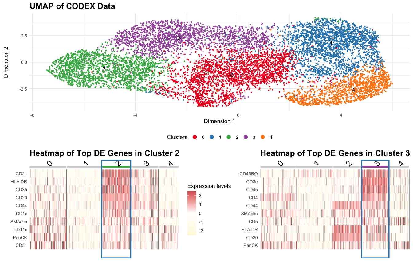
The visualization utilizes UMAP to reduce the high-dimensional CODEX data into a 2D projection, which allows for effective clustering of cells with similar marker expression patterns. Each point in the UMAP plot represents a single cell, and colors indicate different clusters. The presence of five distinct clusters (0-4) represent diverse cell types.

To further explore the molecular identity of Cluster 2 and Cluster 3, heatmaps were generated for their top differentially expressed (DE) genes respectively. These heatmaps display gene expression levels across all clusters, highlighting genes that are highly upregulated in the clusters of interest. The red coloration in the heatmap corresponds to high gene expression, while white regions indicate low or no expression. The blue boxes outline Clusters 2 and 3, allowing for a clearer focus on their expression patterns.

Cluster 2 (green in the UMAP plot) exhibits strong expression of CD20, CD21, CD35, and HLA-DR, all of which are hallmark B-cell markers. CD20 and CD21 are key surface proteins present on mature B cells, while CD35 plays a role in immune complex clearance. Additionally, HLA-DR, a major histocompatibility complex (MHC) class II molecule, suggests the presence of antigen-presenting B cells. Given that B cells are primarily located in the Follicular Zone of the White Pulp in the spleen based on previous research (Pabst & Mebius, 2007).

Cluster 3 (purple in UMAP) is characterized by high expression of CD3e, CD4, CD5, and CD45RO, which are signature markers of T cells. CD3e and CD4 are hallmarks of helper T cells, while CD5 is associated with T-cell receptor (TCR) signaling. Furthermore, CD45RO is a memory T-cell marker, indicating that these cells may be long-lived antigen-experienced T cells (Kisseberth & McEntee, 2006).

In conclusion, the tissue structure is likely to be white pulp; cluster 2 is likely B cells; and cluster 3 is likely T cells.

Pabst, R., & Mebius, R. E. (2007). Anatomical compartmentalization of immune responses in the spleen. Trends in Immunology, 28(8), 386-392.

Kisseberth, W. C., & McEntee, M. C. (2006). Diseases of the spleen. In S. J. Birchard & R. G. Sherding (Eds.), Saunders Manual of Small Animal Practice (3rd ed., pp. 272–282). W.B. Saunders. https://doi.org/10.1016/B0-72-160422-6/50027-9

library(Seurat)
library(ggplot2)
library(patchwork)
library(dplyr)

# IMPORT 
data = read.csv('Users/yiyang/Downloads/codex_spleen_3.csv.gz')
metadata <- data[, c("x","y","area")]
rownames(metadata) <- data$X
data <- data[, !colnames(data) %in% c("X","y","x","area")]
# QUALITY CONTROL
metadata$total_counts <- rowSums(data)
low_threshold <- quantile(metadata$total_counts, 0.01)
high_threshold <- quantile(metadata$total_counts, 0.99)
min_area <- quantile(metadata$area, 0.01) 
max_area <- quantile(metadata$area, 0.99)
keep_cells <- which(
  metadata$total_counts >= low_threshold & 
    metadata$total_counts <= high_threshold &
    metadata$area >= min_area & 
    metadata$area <= max_area
)
data_qc <- data[keep_cells, ]
metadata_qc <- metadata[keep_cells, ]
# ANALYSIS
seurat_obj <- CreateSeuratObject(counts = t(data_qc), meta.data = metadata_qc)
seurat_obj <- NormalizeData(seurat_obj)
seurat_obj <- FindVariableFeatures(seurat_obj, selection.method = "vst", nfeatures = 2000)
seurat_obj <- ScaleData(seurat_obj)
seurat_obj <- RunPCA(seurat_obj, features = VariableFeatures(object = seurat_obj))
seurat_obj <- RunUMAP(seurat_obj, dims = 1:20)
seurat_obj <- FindNeighbors(seurat_obj, dims = 1:20)
seurat_obj <- FindClusters(seurat_obj, resolution = 0.2)
title_theme <- theme(plot.title = element_text(size = 16, face = "bold"))
Idents(seurat_obj) <- "seurat_clusters"
cluster_colors <- c("0" = "#E41A1C", "1" = "#377EB8", "2" = "#4DAF4A", 
                    "3" = "#984EA3", "4" = "#FF7F00", "5" = "#FFFF33", 
                    "6" = "#A65628", "7" = "#F781BF", "8" = "#999999")
p1 = DimPlot(seurat_obj, reduction = "umap", label = TRUE, pt.size = 0.5) +
  scale_color_manual(values = cluster_colors, name = "Clusters") +
  ggtitle("UMAP of CODEX Data") +
  labs(x ="Dimension 1", y = "Dimension 2") +
  theme_minimal() + theme(legend.position = "bottom") + title_theme 
  
# IDENTIFY CLUSTERS
cluster_of_interest <- "2"  
markers_cluster <- FindMarkers(seurat_obj, ident.1 = cluster_of_interest, min.pct = 0.25, logfc.threshold = 0.25)
top_genes <- rownames(markers_cluster[order(markers_cluster$avg_log2FC, decreasing = TRUE),])[1:10] 
cluster_colors_2 <- rep("#D3D3D3", length(unique(Idents(seurat_obj)))) 
names(cluster_colors_2) <- levels(seurat_obj)  
cluster_colors_2["2"] <- "#4DAF4A"
p2 = DoHeatmap(seurat_obj, features = top_genes, group.colors = cluster_colors_2) +
  ggtitle("Heatmap of Top DE Genes in Cluster 2") + 
  scale_fill_gradientn(colors = c("#FFF8DC", "white","#CD5555"), 
                       name = "Expression levels") +
  scale_color_manual(name = "Clusters", values = cluster_colors) +
  annotate("rect", xmin = 4700, xmax = 6600, ymin = -Inf, ymax = Inf, 
           color = "#377EB8", size = 1, fill = NA) +
  guides(color = "none") + title_theme 

cluster_of_interest <- "3"  
markers_cluster <- FindMarkers(seurat_obj, ident.1 = cluster_of_interest, min.pct = 0.25, logfc.threshold = 0.25)
top_genes <- rownames(markers_cluster[order(markers_cluster$avg_log2FC, decreasing = TRUE),])[1:10] 
cluster_colors_3 <- rep("#D3D3D3", length(unique(Idents(seurat_obj)))) 
names(cluster_colors_3) <- levels(seurat_obj)  
cluster_colors_3["3"] <- "#984EA3"  
p3 = DoHeatmap(seurat_obj, features = top_genes, group.colors = cluster_colors_3) +
  ggtitle("Heatmap of Top DE Genes in Cluster 3") + 
  scale_fill_gradientn(colors = c("#FFF8DC", "white","#CD5555"), 
                       name = "Expression levels") +
  scale_color_manual(name = "Clusters", values = cluster_colors) +
  annotate("rect", xmin = 6620, xmax = 8400, ymin = -Inf, ymax = Inf, 
           color = "#377EB8", size = 1, fill = NA) +
  theme(legend.position = "none") + title_theme

p1 / (p2 | p3)