Tissue structure identification for spleen CODEX Dataset

Description of analysis

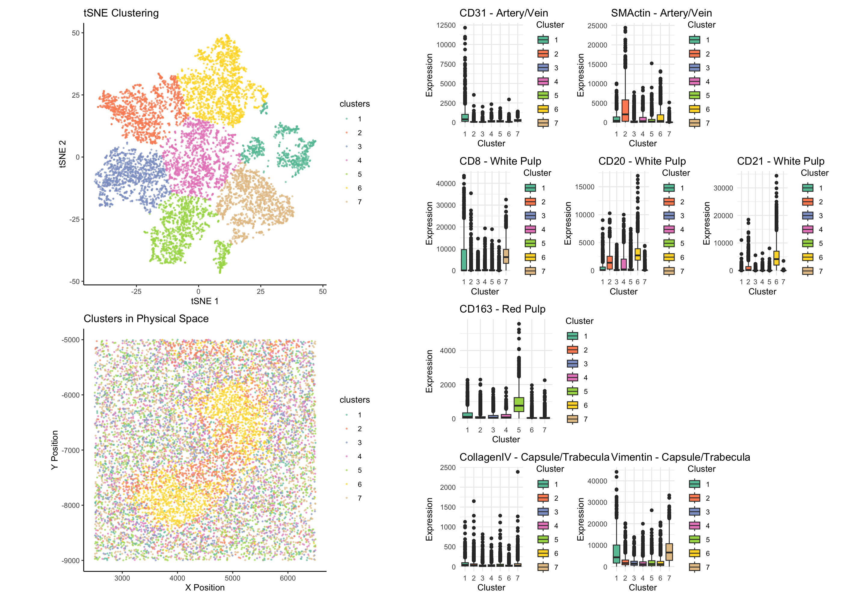
Through a combination of spatial clustering and differential expression analysis, I identified clusters 2 and 6 as the primary contributors to the tissue structure in our CODEX dataset. These clusters exhibit a dense, centralized organization, suggesting their involvement in a well-defined anatomical structure. Given the provided classification options—Artery/Vein, White Pulp, Red Pulp, and Capsule/Trabecula—our analysis supports the conclusion that the observed structure corresponds to white pulp of the spleen. To validate this classification, I examined differentially expressed proteins in clusters 2 and 6, focusing on markers associated with distinct splenic compartments: White Pulp Markers (CD8, CD20, CD21) CD8 is a well-established marker for cytotoxic T cells, which are abundant in the periarteriolar lymphoid sheath (PALS) of the white pulp, surrounding central arterioles (Mebius & Kraal, 2005). CD20 marks mature B cells, which are densely packed in the B-cell follicles of the white pulp (Steiniger, 2015). CD21 is a marker for follicular dendritic cells, which play a critical role in organizing B-cell zones within the white pulp (Steiniger et al., 2006). Artery/Vein Markers (CD31, SMActin) CD31 (PECAM-1) is a marker for endothelial cells, which line blood vessels, and SMActin (α-Smooth Muscle Actin) is a marker of vascular smooth muscle cells (Zhou et al., 2014). Neither marker was significantly expressed in clusters 2 and 6, ruling out vascular structures. Red Pulp Marker (CD163) CD163 is a macrophage marker highly expressed in the sinusoidal macrophages of the red pulp, which are involved in erythrocyte turnover (Kurosawa et al., 2021). The lack of CD163 expression in these clusters indicates that they do not correspond to red pulp. Capsule/Trabecula Markers (Collagen IV, Vimentin) Collagen IV is a component of the basement membrane and is highly expressed in splenic capsule and trabeculae (Wheater et al., 2019). Vimentin is an intermediate filament protein that marks mesenchymal-derived cells and is found in fibroblastic reticular cells of the capsule and trabeculae (Thiele et al., 2012). Minimal expression of these markers suggests that clusters 2 and 6 are not part of the capsule or trabeculae.

The spatial distribution of clusters 2 and 6 forms a compact, centralized structure, characteristic of white pulp, which appears as discrete lymphoid nodules surrounding central arterioles (Steiniger, 2015). This pattern is distinct from the more dispersed nature of red pulp macrophages or the linear alignment of capsule/trabeculae. Based on the bhigher expression of CD20 and CD21 in cluster 2 and 6, and from the spatial clustering, I classify this structure as white pulp, rahter than red pulp, atery/vein, or capsule/trabecula.

References

[1]Mebius, R. E., & Kraal, G. (2005). Structure and function of the spleen. Nature Reviews Immunology, 5(8), 606–616 [2]Steiniger, B. S. (2015). Human spleen microanatomy: Why mice do not suffice. Blood, 125(13), 2039–2048. [3]Steiniger, B. S., Barth, P., & Hellinger, A. (2006). The perifollicular and marginal zones of the human splenic white pulp: Do fibroblasts guide lymphocyte immigration? The American Journal of Pathology, 169(2), 651–664 [4]Zhou, B., Wang, D. D., Qian, H. Y., & Wang, H. (2014). The roles of endothelial cell adhesion molecules in atherosclerosis. Molecular Medicine Reports, 9(3), 1049–1057. [5]Kurosawa, S., Kanegane, H., Imai, K., & Yachie, A. (2021). Role of macrophages in the red pulp of human spleen. Frontiers in Immunology, 12, 751228 [6]Wheater, P. R., Burkitt, H. G., & Daniels, V. G. (2019). Functional Histology: A Text and Colour Atlas. Elsevier.

## Load required libraries
library(ggplot2)
library(Rtsne)
library(ggrepel)
library(dplyr)
library(patchwork)
library(RColorBrewer)

# Load dataset
data <- read.csv('~/Desktop/genomic-data-visualization-2025/data/codex_spleen_3.csv.gz',
                 row.names = 1)

# Extract relevant data
position <- data[, 1:2]
cell_area <- data[, 3]
gexp <- data[, 4:31]

# Normalize protein expression using a modified log transformation
norm_expr <- log1p(gexp / rowSums(gexp) * mean(rowSums(gexp))+1)

# Perform PCA
top_pcs <- prcomp(gexp, center = TRUE, scale. = TRUE)

# Run tSNE on first 15 PCs
set.seed(42)
tsne_results <- Rtsne(top_pcs$x[, 1:15], perplexity = 30, verbose = TRUE, max_iter = 1000)$Y
tsne_df <- data.frame(X1 = tsne_results[, 1], X2 = tsne_results[, 2])

# Determine optimal clusters using silhouette analysis
library(cluster)
k_values <- 2:10
sil_scores <- sapply(k_values, function(k) {
  km_res <- kmeans(tsne_results, centers = k, nstart = 25)
  mean(silhouette(km_res$cluster, dist(tsne_results))[, 3])
})
optimal_k <- k_values[which.max(sil_scores)]

# Perform K-means clustering
set.seed(42)
kmeans_result <- kmeans(tsne_results, centers = optimal_k, nstart = 50)
clusters <- factor(kmeans_result$cluster)

# Define color palette for clusters
cluster_palette <- brewer.pal(optimal_k, "Set2")

# Plot tSNE clustering
p1 <- ggplot(tsne_df, aes(X1, X2, color = clusters)) +
  geom_point(alpha = 0.6, size = 0.5) +
  scale_color_manual(values = cluster_palette) +
  theme_classic() +
  labs(title = "tSNE Clustering", x = "tSNE 1", y = "tSNE 2")
p1 <- p1 + coord_fixed(ratio = 1/1)

# Plot clusters in physical space
p2 <- ggplot(data.frame(position, clusters), aes(x = x, y = y, color = clusters)) +
  geom_point(alpha = 0.6, size = 0.5) +
  scale_color_manual(values = cluster_palette) +
  theme_classic() +
  labs(title = "Clusters in Physical Space", x = "X Position", y = "Y Position")
p2 <- p2 + coord_fixed(ratio = 1/1)


# Extract expression data for clusters 6 and 2
cluster_6_cells <- which(clusters == 6)
cluster_2_cells <- which(clusters == 2)

expr_cluster_6 <- gexp[cluster_6_cells, ]
expr_cluster_2 <- gexp[cluster_2_cells, ]

# Perform Wilcoxon rank-sum test for each protein
p_values <- apply(gexp, 2, function(protein_expr) {
  wilcox.test(protein_expr[cluster_6_cells], protein_expr[cluster_2_cells])$p.value
})

# Adjust p-values using the Benjamini-Hochberg method
adj_p_values <- p.adjust(p_values, method = "BH")

# Identify significantly differentially expressed proteins
signif_proteins <- names(adj_p_values[adj_p_values < 0.05])

# Display significant proteins
print("Significantly differentially expressed proteins:")
print(signif_proteins)

# Define the Set2 palette for all clusters
cluster_palette <- brewer.pal(optimal_k, "Set2")

# Marker gene list by tissue structure
markers <- list(
  "Artery/Vein" = c("CD31", "SMActin"),
  "White Pulp" = c("CD8", "CD20", "CD21"),
  "Red Pulp" = c("CD163"),
  "Capsule/Trabecula" = c("CollagenIV", "Vimentin")
)

# Convert the markers list to a data frame for easy plotting
marker_df <- data.frame(
  Marker = unlist(markers),
  Tissue = rep(names(markers), sapply(markers, length))
)

# Function to plot expression by cluster for each marker
marker_expr_plot_all <- function(marker, tissue) {
  data_to_plot <- data.frame(Expression = gexp[, marker],
                             Cluster = clusters)
  
  ggplot(data_to_plot, aes(x = Cluster, y = Expression, fill = Cluster)) +
    geom_boxplot() +
    labs(title = marker,
         x = "Cluster", y = "Expression") +
    theme_minimal() +
    scale_fill_manual(values = cluster_palette) +
    ggtitle(paste(marker, "-", tissue))
}

# Generate plots for all markers, grouped by tissue structure
marker_plots <- lapply(1:nrow(marker_df), function(i) {
  marker_expr_plot_all(marker_df$Marker[i], marker_df$Tissue[i])
})

# Get unique tissues (e.g., artery, vein, etc.)
unique_tissues <- unique(marker_df$Tissue)

# Organize plots by tissue structure
tissue_plots <- lapply(unique_tissues, function(tissue) {
  # Get markers corresponding to the tissue
  tissue_markers <- marker_df$Marker[marker_df$Tissue == tissue]
  tissue_plots <- lapply(tissue_markers, function(marker) {
    marker_expr_plot_all(marker, tissue)
  })
  
  # Combine plots for this tissue structure (e.g., artery/vein)
  wrap_plots(tissue_plots, ncol = 3) + plot_annotation(title = tissue)
})

# Combine all tissue plots
p3 <- wrap_plots(tissue_plots, ncol = 1) + 
  plot_annotation(title = "Marker Gene Expression by Tissue Structure and Cluster")


print(p3)

#patchwork
patch <- (p1 / p2) | p3 + plot_layout(widths = c(1, 3))
print(patch)