Identifying the Tissue

Description
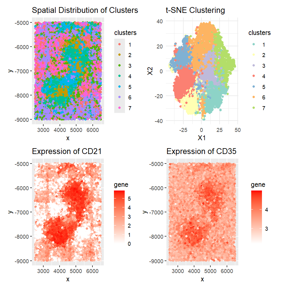
CD21 and CD35 are highly expressed in the White pulp (2) of the spleen. These markers are typically associated with follicular dendritic cells (FDCs) and B cells, both of which are predominantly found in the white pulp, particularly within B cell follicles and germinal centers.
To reach this conclusion, I first normalized the data and applied k-means clustering. Upon plotting the spatial distribution of the cells, I observed that cluster 3 exhibited a distinct spatial pattern. To further validate this, I used t-SNE, which preserves local distances and patterns, and confirmed the cluster’s spatial arrangement.
Next, I conducted a one-sided Wilcoxon test to identify genes that were significantly upregulated in cluster 3. CD21 and CD35 emerged as the most highly regulated genes. I confirmed their high expression in specific regions through expression plots, supporting the hypothesis that cluster 3 represents the white pulp of the spleen, where B cells and FDCs are most concentrated.
Source: https://www.nature.com/articles/nri1669
Code (paste your code in between the ``` symbols)
1
2
3
4
5
6
7
8
9
10
11
12
13
14
15
16
17
18
19
20
21
22
23
24
25
26
27
28
29
30
31
32
33
34
35
36
37
38
39
40
41
42
43
44
45
46
47
48
49
50
51
52
53
54
55
56
57
58
59
60
61
62
63
64
65
66
67
68
69
70
71
72
73
74
75
76
77
78
79
80
81
82
83
84
85
86
87
88
library(ggplot2)
library(patchwork)

data <- read.csv('genomic-data-visualization-2025/data/codex_spleen_3.csv.gz', row.names = 1)
print(data)

pos <- data[,]
exp <- data[, 3:ncol(data)]
head(pos)
head(exp)
dim(exp)

# Normalize the expression data
norm <- log10(exp/rowSums(exp) * 1e6 + 1)
print(norm[1:5, 1:5])

#finding the best cluster:
set.seed(42)
ks = c(5,6,7,8,9,10)
#around ks = 7 is the elbow
totw <- sapply(ks, function(k) {
  print(k)
  com <- kmeans(gexp, centers=k)
  return(com$tot.withinss)
})
plot(ks, totw, main="Elbow Plot for Optimal k", xlab="Number of Clusters", ylab="Total Within-Cluster Sum of Squares")

kmeans_result <- kmeans(norm, centers = 7)
clusters <- kmeans_result$cluster
head(clusters)

# Prepare data for plotting
colnames(pos) <- c("x", "y")
df <- data.frame(pos, clusters = as.factor(clusters))

# Create scatter plot using ggplot2
g1 <- ggplot(df, aes(x = x, y = y, color = clusters)) +
  geom_point() +
  ggtitle("Spatial Distribution of Clusters")
g1
#from the spatial dynamics, we can see that cluster 3 is spatialy together, with cluster four mainly surrounding cluster 3

#verifying with a tsne plot
emb <- Rtsne::Rtsne(norm)
df <- data.frame(emb$Y, clusters)
df$clusters <- as.factor(df$clusters)

# Plot with distinct colors for each cluster
g4 <- ggplot(df, aes(x = X1, y = X2, color = clusters)) +
  geom_point() +
  scale_color_brewer(palette = "Set3") +  # Distinct colors for each cluster
  ggtitle("t-SNE Clustering") +
  theme_minimal()
g4

#find most upregulated gene within cluster 3:
ct1 <- names(clusters)[which(clusters == 3)]
ctother <- names(clusters)[which(clusters != 3)]
results <- sapply(colnames(norm), function(i) {
  wilcox.test(norm[ct1, i], norm[ctother, i],alternative = "greater")$p.value ## one sided test
})
names(results) <- colnames(norm)
sort(results[results < 0.05/ncol(norm)])
#CD21 and CD35 are the top two most upregulated genes

print(data)

df <- data.frame(data, gene=norm[,'CD21'])
g2 <- ggplot(df,aes(x=x, y=y, col=gene)) +
  geom_point() +
  scale_color_gradient(low = "white", high = "red") +
  ggtitle("Expression of CD21")
g2
#CD21 is most expressed in the areas where cluster 3 is expressed

df <- data.frame(data, gene=norm[,'CD35'])
g3 <- ggplot(df,aes(x=x, y=y, col=gene)) +
  geom_point() +
  scale_color_gradient(low = "white", high = "red") +
  ggtitle("Expression of CD35")
g3
#Although less than CD21, CD35 is also similairly is expressed in the areas where cluster 3 is expressed

#final patchwork display
final_plot <- (g1 + g4 ) / (g2 + g3)
print(final_plot)