Cluster characterization in sequencing-based spatial transcriptomics

Homework 5
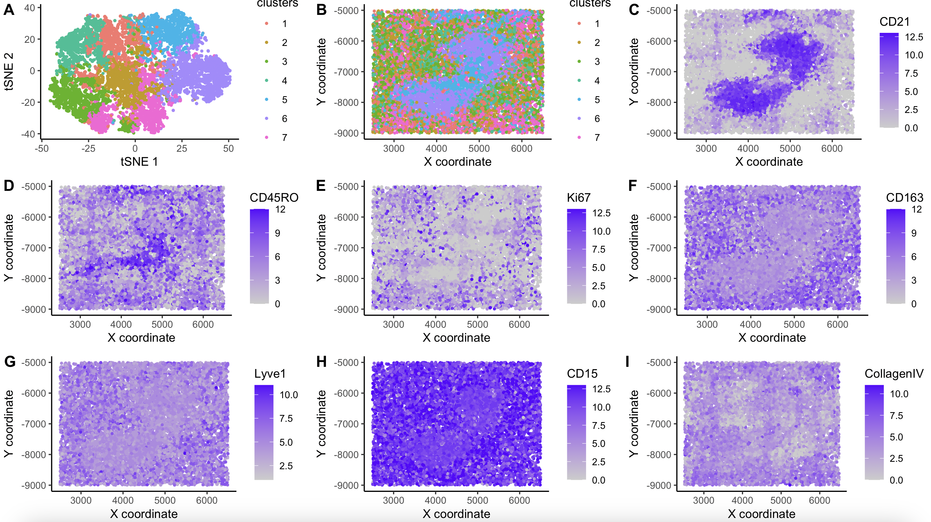
Co-detection by indexing (CODEX) data from spleen tissue assessing 28 proteins was analized.As a QC step, data was normalized: raw counts were divided by total spot counts, multiplied by the scale factor 10000 and the result was log transformed. Likewise, data was scaled to prevent proteins with the highest mean from contributing the most to the variabliity. PCA was performed to reduce the dimensionality of the dataset. after looking at “Elbow plot” 8 PCs were selected for furthe analysis. Then, k-means was used to find clusters of cells, using PCs as input. After plotting “total withinness” I selected k=7. Lastly, t-SNE was used for visual purposes and calculated using PCs as input, were spots with similar proteome appear together (Figure A).
Clusters were visualized in their spatial location(Figure B). Strikingly, clusters 5 and 6 had a very distinctive pattern at the center of the slide, whereas the rest of the clusters were dispersed and did not have a marked pattern. Then, differentialy expressed proteins were calculated for every cluster. Cluster 5 had a high expression of T cell markers (CD45RO, CD3e, CD4, CD21, CD45) and cluster 6 had B cell markers (CD21, HLA-DR, CD20) and CD4 (most likely coming from CD4+ helper cells that interact with B-cells in the germinal centers of the spleen). This data suggests, that clusters 5 and 6 correspond to the White Pulp of the spleen[1, 3].
On the other hand, the rest of the clusters showed markers rather expressed in the Red Pulp of the spleen[1,2]: 1 - Ki67 (highest FC=0.94806589) Proliferation marker, cells of the Red Pulp undergoing turnover and renewal 2 - CD163, CD68 (macrophages) [2] 3 - CD8, Lyve1 (vascular structures in the Red Pulp) 4 - CD15 (highest FC=0.30174821) (neutrophils and myeloid cells) 7 - Podoplanin, CollagenIV
UMAP plots showing the Gene expression of important marker proteins are showing to help understand the spleen tissue: CD21 (Figure C:white pulp Bcells), CD45RO (Figure D:white pulp Tcells), Ki67 (Figure E:renewing red pulp), CD163 (Figure F:red pulp macrophages), Lyve1 (Figure G:vascular red pulp), CD15 (Figure H: red pulp neutrophils) and CollagenIV (Figure I: red pulp structure).
References:
- Borch, W. R., Aguilera, N. S., Brissette, M. D., O’Malley, D. P., & Auerbach, A. (2019). Practical applications in immunohistochemistry: an immunophenotypic approach to the spleen. Archives of pathology & laboratory medicine, 143(9), 1093-1105.
- Nagelkerke, S. Q., Bruggeman, C. W., Den Haan, J. M., Mul, E. P., Van Den Berg, T. K., Van Bruggen, R., & Kuijpers, T. W. (2018). Red pulp macrophages in the human spleen are a distinct cell population with a unique expression of Fc-γ receptors. Blood advances, 2(8), 941-953.
- Cheng, H. W., Onder, L., Novkovic, M., Soneson, C., Lütge, M., Pikor, N., … & Ludewig, B. (2019). Origin and differentiation trajectories of fibroblastic reticular cells in the splenic white pulp. Nature communications, 10(1), 1739.
Code
1
2
3
4
5
6
7
8
9
10
11
12
13
14
15
16
17
18
19
20
21
22
23
24
25
26
27
28
29
30
31
32
33
34
35
36
37
38
39
40
41
42
43
44
45
46
47
48
49
50
51
52
53
54
55
56
57
58
59
60
61
62
63
64
65
66
67
68
69
70
71
72
73
74
75
76
77
78
79
80
81
82
83
84
85
86
87
88
89
90
91
92
93
94
95
96
97
98
99
100
101
102
103
104
105
106
107
108
109
110
111
112
113
114
115
116
117
118
119
120
121
122
# - Import libraries
library(ggplot2)
library(tidyverse)
library(cowplot)
library(patchwork)
library(Rtsne)
library(DESeq2)
library(STdeconvolve)

# - Read data
file <- '/Users/kmlanderos/Documents/Johns_Hopkins/Spring_2025/Genomic_Data_Visualization/genomic-data-visualization-2025/data/codex_spleen_3.csv.gz'
data <- read.csv(file, row.names=1)
gexp<-data[,4:ncol(data)]
gexp<-gexp[,colSums(gexp)!=0] # Remove proteins with no expression across cells
set.seed(100)

# - Normalize and scale data first
norm_data<-log2(10000*gexp/rowSums(gexp) + 1)
scaled_data<-scale(norm_data)

# - PCA
pca <- prcomp(scaled_data)
# Make Scree plot to choose PCs: Elbow PLOT
n_pcs=8
df_tmp <- data.frame(pc=1:n_pcs, sdev=pca$sdev[1:n_pcs])
ggplot(df_tmp, aes(x=pc, y=sdev)) + geom_point()

# - K means
# Try many ks
ks<-2:10
tot_withinss<- sapply(ks, function(k){
  print(k)
  res<-kmeans(gexp, centers=k)
  return(res$tot.withinss)
})
# Plot withinness
plot(ks, tot_withinss)
k=7
res<-kmeans(pca$x[,1:8], centers=k)
clusters<- as.factor(res$cluster)
# - t-SNE
tsne <- Rtsne(pca$x[,1:8])

popo <- data.frame(clusters, X_coord=data$x, Y_coord=data$y, pca$x[,1:3], tSNE_1= tsne$Y[,1], tSNE_2= tsne$Y[,2])
ggplot(popo, aes(x=tSNE_1, y=tSNE_2, color=clusters)) + geom_point(size=0.1)

# - DEGs
get_degs <- do.call(rbind, lapply(levels(clusters), function(cluster){ # cluster=1
  condition1_cells <- names(clusters)[clusters == cluster]
  condition2_cells <- names(clusters)[clusters != cluster]

  # Compute means
  clust_mean <- colMeans(norm_data[condition1_cells, , drop=FALSE])
  rest_mean <- colMeans(norm_data[condition2_cells, , drop=FALSE])

  # Perform Wilcoxon test for all proteins
  cluster_comparisons <- apply(norm_data, 2, function(protein_expr) {
    out <- wilcox.test(protein_expr[condition1_cells], protein_expr[condition2_cells], alternative='two.sided')
    return(out$p.value)
  })

  # Compute log2 fold change (adding pseudocount to prevent division by zero)
  log2FC <- log2((clust_mean + 1e-6) / (rest_mean + 1e-6))

  # Create DEG dataframe
  proteins_df <- data.frame(
    cluster = cluster,
    protein = names(clust_mean),
    clust_mean = clust_mean,
    rest_mean = rest_mean,
    log2FC = log2FC,
    p_value = cluster_comparisons,
    p_adj = p.adjust(cluster_comparisons, method = "BH")
  ) %>% mutate(
    log_p_adj = -log10(p_adj),
    significance = case_when(
      log2FC > 0.50 & p_adj < 0.05 ~ "Upregulated",
      log2FC < -0.50 & p_adj < 0.05 ~ "Downregulated",
      TRUE ~ "Not Significant"
    )
  )

  return(proteins_df)
}))

# Top proteins per cluster
top_degs_per_cluster <- get_degs %>% filter (p_adj < 0.05 & log2FC>0) %>%
  group_by(cluster) %>%  # Group by cluster
  arrange(desc(log2FC)) %>%  # Sort by adjusted p-value within each cluster
  slice_head(n = 5) %>%  # Select the top 5 DEGs per cluster
  ungroup() %>% data.frame()
top_degs_per_cluster


# - Plots
# Data Frame
df <- data.frame(clusters, X_coord=data$x, Y_coord=data$y, pca$x[,1:3], tSNE_1= tsne$Y[,1], tSNE_2= tsne$Y[,2], celltype_singleR=singleR_results$labels)

# Plot Panel A
p1<-ggplot(df, aes(x=tSNE_1, y=tSNE_2, color=clusters)) + geom_point(size=0.7) + labs(x="tSNE 1", y="tSNE 2") + theme_classic()
# Plot Panel B
p2<-ggplot(df, aes(x=X_coord, y=Y_coord, color=clusters)) +
labs(x="X coordinate", y="Y coordinate") + geom_point(size=0.7) + theme_classic()
p3<-ggplot(df, aes(x=X_coord, y=Y_coord, color=norm_data[,"CD21"])) + geom_point(size=0.7) + scale_colour_gradient(low = "gray80", high = "#5800FF") +
labs(x="X coordinate", y="Y coordinate", color="CD21") + theme_classic()
p4<-ggplot(df, aes(x=X_coord, y=Y_coord, color=norm_data[,"CD45RO"])) + geom_point(size=0.7) + scale_colour_gradient(low = "gray80", high = "#5800FF") +
labs(x="X coordinate", y="Y coordinate", color="CD45RO") + theme_classic()

# -Gex UMAP Plots
p5<-ggplot(df, aes(x=X_coord, y=Y_coord, color=norm_data[,"Ki67"])) + geom_point(size=0.7) + scale_colour_gradient(low = "gray80", high = "#5800FF") +
labs(x="X coordinate", y="Y coordinate", color="Ki67") + theme_classic()
p6<-ggplot(df, aes(x=X_coord, y=Y_coord, color=norm_data[,"CD163"])) + geom_point(size=0.7) + scale_colour_gradient(low = "gray80", high = "#5800FF") +
labs(x="X coordinate", y="Y coordinate", color="CD163") + theme_classic()
p7<-ggplot(df, aes(x=X_coord, y=Y_coord, color=norm_data[,"Lyve1"])) + geom_point(size=0.7) + scale_colour_gradient(low = "gray80", high = "#5800FF") +
labs(x="X coordinate", y="Y coordinate", color="Lyve1") + theme_classic()
p8<-ggplot(df, aes(x=X_coord, y=Y_coord, color=norm_data[,"CD15"])) + geom_point(size=0.7) + scale_colour_gradient(low = "gray80", high = "#5800FF") +
labs(x="X coordinate", y="Y coordinate", color="CD15") + theme_classic()
p9<-ggplot(df, aes(x=X_coord, y=Y_coord, color=norm_data[,"CollagenIV"])) + geom_point(size=0.7) + scale_colour_gradient(low = "gray80", high = "#5800FF") +
labs(x="X coordinate", y="Y coordinate", color="CollagenIV") + theme_classic()

plot_grid(p1, p2, p3, p4, p5, p6, p7, p8, p9, labels = "AUTO")