Identification of White Pulp Tissue Structure in Spleen CODEX Data

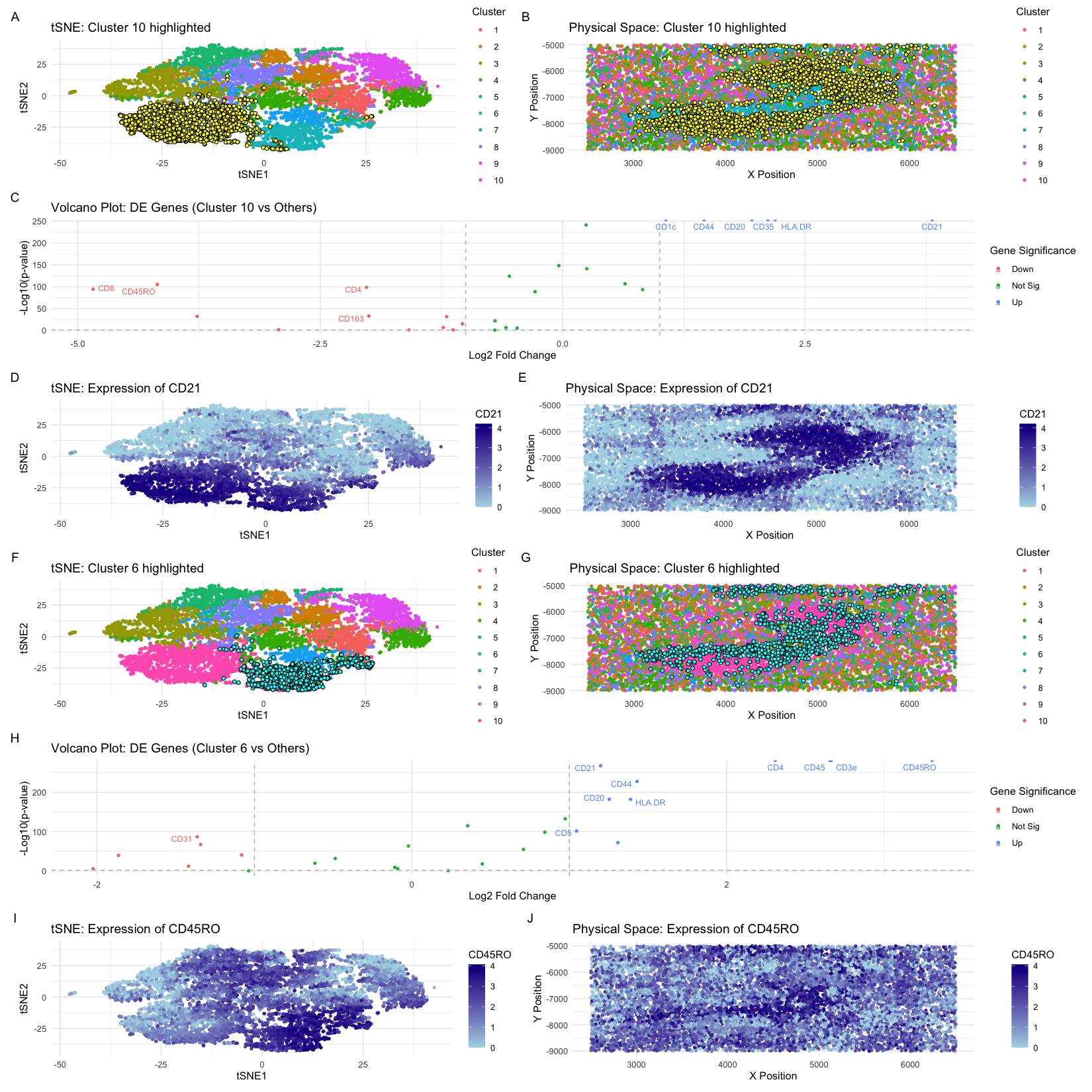
Here I perform clustering and differential expression analysis on a CODEX data set obtained from a spleen sample. Following an identification of the ideal 10 k-means clusters, I visualized the clusters in tSNE dimensionality reduced space and in physical space. Isolating clusters and performing differential analysis, I identified two clusters, 10 and 6, that I found to be particularly interesting for their upregulated expression of CD21 and CD45RO, respectively. For each, I visualize the expression of the gene in tSNE space and physical space, which confirms their expression within the cluster visualizations prior. Here, I will support the conclusion that cluster 10 is representative of follicular dendritic cells and cluster 6 represents T-lymphocyte-like cells and are supportive that the white pulp tissue structure is represented in the CODEX data.
Cluster 10 shows the upregulated expression of CD21, HLA.DR, and CD35. Follicular dendritic cells have been demonstrated to express the CD21 isoform as one of its cellular markers (Liu et al, 1997). Dendritic cells expressing HLA.DR are often present in follicular fluid (Fainaru et al., 2011). Lastly, CD35 is a protein that is used to identify follicular dendritic cells in lymphoid tissues and are part of the Splenic CD19-CD35+B220+ cells that function as an inducer of follicular dendritic cell network formation (Murakami et al., 2007). All in all,this supports the conclusion that cluster 10 is representative of the follicular dendritic cell type.
Cluster 6 shows the upregulation of CD45RO, CD3e, and CD45 most notably. CD45RO is an antigen present on CD4 T-cells that are specific to the memory family (Devi et al., 2017). CD3e is a glycoprotein that is most abundantly found on the surface of T cells (https://www.ncbi.nlm.nih.gov/gene/916) (CD45 is a marker protein expression on the surface of all T cells and is a crucial component for proper T cell receptor signaling by regulating the activation state of other proteins involved in T cell inactivation (Altin et al., 1997). Furthermore CD45 is often used as the marker for T-cell separation techniques. Thus, I conclude that this cell cluster is representative of the T-cell type.
Thus, I conclude that I have identified two cell types that are representative of the white pulp tissue structure of the spleen. The white pulp of the spleen is a lymphatic tissue that plays a crucial role in the immune system. It is componed mainly of lymphocytes around arteries. This is supported by the upregulation of T-cell markers in cluster 6 (https://www.histology.leeds.ac.uk/lymphoid/lymph_spleen.php#:~:text=White%20pulp%20contains%20lymphoid%20aggregations,helper)%20and%20B%2Dcells.). Additionally, follicles are arranged at the outer cortex near the capsule of lymph nodes and the outer part of the white pulp (https://www.sciencedirect.com/topics/immunology-and-microbiology/follicular-dendritic-cells#:~:text=Follicles%20are%20arranged%20at%20the,of%20the%20tonsils%20and%20PPs.). Specifically, follicular dendritic cells are known to form dense networks in the center of follicles (https://www.sciencedirect.com/topics/immunology-and-microbiology/follicular-dendritic-cells#:~:text=Follicles%20are%20arranged%20at%20the,of%20the%20tonsils%20and%20PPs.) Given, that in cluster 10 I identify the upregulation of several markers that are associated with follicular dendritic cells, I conclude that the cluster is representative of this cell type. Given that both clusters identified represent cell types that are characteristic of the cells within the white pulp, I conclude that this tissue structure is represented in the CODEX data.
Liu et al, 1997: https://pubmed.ncbi.nlm.nih.gov/8996252/ Fainaru et al., 2011: https://www.sciencedirect.com/science/article/pii/S0015028211029141?via%3Dihub Murakami et al., 2007: https://pubmed.ncbi.nlm.nih.gov/17519390/#:~:text=Abstract,to%20initiate%20lymphoid%20follicle%20formation. Altin et al., 19973: https://pubmed.ncbi.nlm.nih.gov/9429890/#:~:text=CD45%20(lymphocyte%20common%20antigen)%20is,CD3%20complex%20and%20CD4/CD8. Devi et al., 2017: https://pmc.ncbi.nlm.nih.gov/articles/PMC5483817/ https://www.ncbi.nlm.nih.gov/gene/916
Code
1
2
3
4
5
6
7
8
9
10
11
12
13
14
15
16
17
18
19
20
21
22
23
24
25
26
27
28
29
30
31
32
33
34
35
36
37
38
39
40
41
42
43
44
45
46
47
48
49
50
51
52
53
54
55
56
57
58
59
60
61
62
63
64
65
66
67
68
69
70
71
72
73
74
75
76
77
78
79
80
81
82
83
84
85
86
87
88
89
90
91
92
93
94
95
96
97
98
99
100
101
102
103
104
105
106
107
108
109
110
111
112
113
114
115
116
117
118
119
120
121
122
123
124
125
126
127
128
129
130
131
132
133
134
135
136
137
138
139
140
141
142
143
144
145
146
147
148
149
150
151
152
153
154
155
156
157
158
159
160
161
162
163
164
165
166
167
168
169
170
171
172
173
174
175
176
177
178
179
180
181
182
183
184
185
186
187
188
189
190
# Libraries
library(ggplot2)
library(Rtsne)
library(patchwork)
library(ggrepel)
library(factoextra) # For WSS plot

# Load Data
file <- "/Users/kevinnguyen/Desktop/genomic-data-visualization-2025/data/codex_spleen_3.csv.gz"
data <- read.csv(file, row.names = 1)

# Extract positional and gene expression data
pos <- data[,1:2]
gexp <- data[,4:31]

# Normalize: scale by library size then log10-transform (add 1 to avoid log(0))
nonzero <- rownames(gexp)[rowSums(gexp) > 0]
pos <- pos[nonzero,]
gexp <- gexp[nonzero,]
totals <- rowSums(gexp)
norm_gexp <- gexp / totals * median(totals)
loggexp <- log10(norm_gexp + 1)

# K-means clustering (10 clusters)
set.seed(2025)
km_out <- kmeans(loggexp, centers = 10)
clusters <- as.factor(km_out$cluster)
names(clusters) <- rownames(loggexp)

# Create position dataframe
pos_df <- data.frame(pos, clusters = clusters)

# tSNE dimensionality reduction
pcs <- prcomp(loggexp)
tsne_res <- Rtsne(pcs$x[, 1:10])
tsne_df <- data.frame(X1 = tsne_res$Y[, 1],
                      X2 = tsne_res$Y[, 2],
                      clusters = clusters)

# Function for differential expression analysis
compute_de_analysis <- function(cluster_id) {
  cells_interest <- names(clusters)[clusters == cluster_id]
  cells_others <- names(clusters)[clusters != cluster_id]

  de_pvals <- sapply(colnames(gexp), function(gene) {
    wilcox.test(loggexp[cells_interest, gene],
                loggexp[cells_others, gene],
                alternative = "two.sided")$p.value
  })
  names(de_pvals) <- colnames(gexp)

  log2fc <- sapply(colnames(gexp), function(gene) {
    mean_in <- mean(gexp[cells_interest, gene])
    mean_out <- mean(gexp[cells_others, gene])
    log2((mean_in + 1e-6) / (mean_out + 1e-6))
  })
  names(log2fc) <- colnames(gexp)

  volcano_df <- data.frame(gene = colnames(gexp),
                           log2FC = log2fc,
                           negLogP = -log10(de_pvals))

  # Annotate significance
  volcano_df$diffexpr <- "Not Sig"
  volcano_df$diffexpr[volcano_df$log2FC > 1 & de_pvals < 0.05] <- "Up"
  volcano_df$diffexpr[volcano_df$log2FC < -1 & de_pvals < 0.05] <- "Down"

  # Label top 10 most significant genes
  sig_genes <- volcano_df[de_pvals < 0.05 & abs(volcano_df$log2FC) > 1, ]
  top_labels <- head(sig_genes[order(-sig_genes$negLogP), ], 10)
  volcano_df$label <- NA
  volcano_df$label[volcano_df$gene %in% top_labels$gene] <- volcano_df$gene[volcano_df$gene %in% top_labels$gene]

  return(volcano_df)
}

# Run DE analysis for Cluster 10 & Cluster 6
volcano_df_10 <- compute_de_analysis("10")
volcano_df_6 <- compute_de_analysis("6")

# Visualization for Cluster 10
cluster_10 <- "10"
p1 <- ggplot(tsne_df, aes(x = X1, y = X2)) +
  geom_point(aes(color = clusters), size = 1) +
  geom_point(data = tsne_df[clusters == cluster_10, ], color = "black", size = 1.5, shape = 21, fill = "yellow") +
  labs(title = paste("tSNE: Cluster", cluster_10, "highlighted"), color = "Cluster", x = "tSNE1", y = "tSNE2") +
  theme_minimal()

p2 <- ggplot(pos_df, aes(x = x, y = y)) +
  geom_point(aes(color = clusters), size = 1) +
  geom_point(data = pos_df[clusters == cluster_10, ], color = "black", size = 1.5, shape = 21, fill = "yellow") +
  labs(title = paste("Physical Space: Cluster", cluster_10, "highlighted"), color = "Cluster", x = "X Position", y = "Y Position") +
  theme_minimal()

p3 <- ggplot(volcano_df_10, aes(x = log2FC, y = negLogP, color = diffexpr)) +
  geom_point(size = 1) +
  geom_text_repel(aes(label = label), size = 3, max.overlaps = Inf) +
  geom_vline(xintercept = c(-1, 1), linetype = "dashed", color = "gray") +
  geom_hline(yintercept = -log10(0.05), linetype = "dashed", color = "gray") +
  labs(title = paste("Volcano Plot: DE Genes (Cluster", cluster_10, "vs Others)"), x = "Log2 Fold Change", y = "-Log10(p-value)", color = "Gene Significance") +
  theme_minimal()


#Select the gene of interest: CD21
up_gene <- "CD21"
cat("Selected gene for analysis:", up_gene, "\n")

tsne_df$gene_expr <- loggexp[, up_gene]
pos_df$gene_expr <- loggexp[, up_gene]

#Panel E: tSNE plot colored by expression of CD21
p4 <- ggplot(tsne_df, aes(x = X1, y = X2)) +
  geom_point(aes(color = gene_expr), size = 1) +
  scale_color_gradient(low = "lightblue", high = "darkblue") +
  labs(title = paste("tSNE: Expression of", up_gene),
       color = up_gene,
       x = "tSNE1",
       y = "tSNE2") +
  theme_minimal()

#Panel F: Physical space plot colored by expression of CD21
p5 <- ggplot(pos_df, aes(x = x, y = y)) +
  geom_point(aes(color = gene_expr), size = 1) +
  scale_color_gradient(low = "lightblue", high = "darkblue") +
  labs(title = paste("Physical Space: Expression of", up_gene),
       color = up_gene,
       x = "X Position",
       y = "Y Position") +
  theme_minimal()


# Visualization for Cluster 6
cluster_6 <- "6"
p6 <- ggplot(tsne_df, aes(x = X1, y = X2)) +
  geom_point(aes(color = clusters), size = 1) +
  geom_point(data = tsne_df[clusters == cluster_6, ], color = "black", size = 1.5, shape = 21, fill = "cyan") +
  labs(title = paste("tSNE: Cluster", cluster_6, "highlighted"), color = "Cluster", x = "tSNE1", y = "tSNE2") +
  theme_minimal()

p7 <- ggplot(pos_df, aes(x = x, y = y)) +
  geom_point(aes(color = clusters), size = 1) +
  geom_point(data = pos_df[clusters == cluster_6, ], color = "black", size = 1.5, shape = 21, fill = "cyan") +
  labs(title = paste("Physical Space: Cluster", cluster_6, "highlighted"), color = "Cluster", x = "X Position", y = "Y Position") +
  theme_minimal()

p8 <- ggplot(volcano_df_6, aes(x = log2FC, y = negLogP, color = diffexpr)) +
  geom_point(size = 1) +
  geom_text_repel(aes(label = label), size = 3, max.overlaps = Inf) +
  geom_vline(xintercept = c(-1, 1), linetype = "dashed", color = "gray") +
  geom_hline(yintercept = -log10(0.05), linetype = "dashed", color = "gray") +
  labs(title = paste("Volcano Plot: DE Genes (Cluster", cluster_6, "vs Others)"), x = "Log2 Fold Change", y = "-Log10(p-value)", color = "Gene Significance") +
  theme_minimal()

#Select the gene of interest: CD45RO
up_gene2 <- "CD45RO"
cat("Selected gene for analysis:", up_gene2, "\n")

tsne_df$gene_expr <- loggexp[, up_gene2]
pos_df$gene_expr <- loggexp[, up_gene2]

#tSNE plot colored by expression of CD45RO
p9 <- ggplot(tsne_df, aes(x = X1, y = X2)) +
  geom_point(aes(color = gene_expr), size = 1) +
  scale_color_gradient(low = "lightblue", high = "darkblue") +
  labs(title = paste("tSNE: Expression of", up_gene2),
       color = up_gene2,
       x = "tSNE1",
       y = "tSNE2") +
  theme_minimal()

#Physical space plot colored by expression of CD45RO
p10 <- ggplot(pos_df, aes(x = x, y = y)) +
  geom_point(aes(color = gene_expr), size = 1) +
  scale_color_gradient(low = "lightblue", high = "darkblue") +
  labs(title = paste("Physical Space: Expression of", up_gene2),
       color = up_gene2,
       x = "X Position",
       y = "Y Position") +
  theme_minimal()


# Combine plots exactly as requested
combined_plot <- (p1 + p2) / (p3) / (p4 + p5) / (p6 + p7) / (p8) / (p9 + p10) + plot_annotation(tag_levels = 'A')

# Print the combined plot
print(combined_plot)