Analysis of Cellular Clusters and Marker Expression in the CODEX Dataset

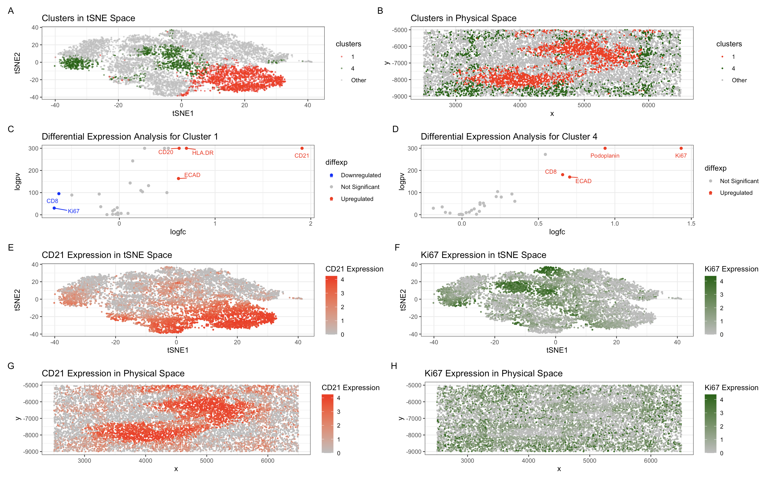
(A) This panel presents the visualization of cellular clusters in tSNE space, where distinct populations (Cluster 1 in red, Cluster 4 in green) are delineated against a background of unclustered cells (gray).
(B) This panel depicts the spatial organization of these clusters in physical tissue space, demonstrating a structured and non-random localization pattern within the tissue architecture.
(C) The left panel illustrates the results of differential expression analysis for Cluster 1, identifying CD21, HLA-DR, ECAD, and CD20 as significantly upregulated markers, consistent with follicular dendritic cells (FDCs) and B-cell populations within lymphoid structures.
(D) The right panel presents differential expression analysis for Cluster 4, highlighting significant upregulation of Podoplanin and Ki-67, indicative of proliferating B cells within a germinal center and possibly stromal support cells involved in the structural organization of lymphoid follicles.
(E) The left panel maps CD21 expression in tSNE space, revealing its selective enrichment in Cluster 1, further supporting the identity of this cluster as a B-cell–rich follicular region with follicular dendritic cell involvement.
(F) The right panel visualizes CD21 expression in physical space, confirming its localized distribution within a distinct anatomical region.
(G, H) The final two panels illustrate Ki-67 expression in both tSNE space and physical space, demonstrating its enrichment in Cluster 4 and its localized proliferation within a specific tissue region. This pattern is consistent with germinal center B cells undergoing rapid clonal expansion.
What Two Distinct Cell Types Are Represented?
The dataset reveals two functionally distinct cell populations:
Cluster 1 differentially upregulates CD21, HLA-DR, and CD20 and is therefore highly indicative of a B cell population, as these markers are characteristic of various stages of B cell development and activation. CD20 (MS4A1) is a well-established marker of mature B cells, including naive and memory B cells, but is absent in plasma cells. CD21 (CR2) is expressed on follicular and germinal center B cells, playing a crucial role in B cell receptor (BCR) signaling and immune complex binding. HLA-DR, a major histocompatibility complex (MHC) class II molecule, is upregulated in antigen-presenting cells (APCs), including B cells, facilitating antigen presentation to CD4+ T cells. The co-expression of these three markers suggests that the cluster represents a mature, antigen-experienced B cell population
Cluster 4 differentially upregulates Ki67 (MKI67), Podoplanin (PDPN), and E-Cadherin (ECAD/CDH1) is indicative of a highly proliferative epithelial cell population. Ki67 marks active cell division, suggesting rapid growth, while E-Cadherin is a hallmark of epithelial identity, maintaining cell-cell adhesion. Podoplanin, though more commonly associated with mesenchymal and lymphatic cells, can also be expressed in certain epithelial contexts, particularly in proliferating or transitioning epithelial cells.
Tissue Identity
The presence of a B cell-rich cluster (upregulating CD21, HLA-DR, and CD20) strongly suggests that this sample is from the white pulp of the spleen, as the white pulp is the primary site of B cell localization and activation within the spleen. The spleen’s white pulp is organized into B cell follicles and germinal centers, where B cells undergo maturation, antigen presentation, and immune responses. The identification of a proliferative epithelial population (upregulating Ki67, Podoplanin, and E-Cadherin) further supports this conclusion, as the spleen’s capsule and trabeculae, which contain mesothelial and stromal cells, are adjacent to the white pulp and may exhibit epithelial proliferation during immune activation or tissue remodeling.
References:
https://pmc.ncbi.nlm.nih.gov/articles/PMC4479725/ https://pmc.ncbi.nlm.nih.gov/articles/PMC3439854/ https://www.proteinatlas.org/ENSG00000204287-HLA-DRA https://www.proteinatlas.org/ENSG00000117322-CR2 https://www.proteinatlas.org/ENSG00000156738-MS4A1 https://www.proteinatlas.org/ENSG00000148773-MKI67 https://www.proteinatlas.org/ENSG00000162493-PDPN https://www.proteinatlas.org/ENSG00000039068-CDH1
1
2
3
4
5
6
7
8
9
10
11
12
13
14
15
16
17
18
19
20
21
22
23
24
25
26
27
28
29
30
31
32
33
34
35
36
37
38
39
40
41
42
43
44
45
46
47
48
49
50
51
52
53
54
55
56
57
58
59
60
61
62
63
64
65
66
67
68
69
70
71
72
73
74
75
76
77
78
79
80
81
82
83
84
85
86
87
88
89
90
91
92
93
94
95
96
97
98
99
100
101
102
103
104
105
106
107
108
109
110
111
112
113
114
115
116
117
118
119
120
121
122
123
124
125
126
127
128
129
130
131
132
133
134
135
136
137
138
139
140
141
142
143
144
145
146
147
148
149
150
151
152
153
154
155
156
157
158
159
160
161
162
163
164
165
166
167
168
169
170
171
172
173
174
175
176
177
178
library(ggplot2)
library(patchwork)
library(Rtsne)
library(ggrepel)
library(dplyr)
library(cluster)
library(reshape2)

# Load dataset
codex_file <- 'codex_spleen_3.csv.gz'
codex_data <- read.csv(codex_file, row.names = 1)

codex_data[1:10, 1:10]

# Separate spatial coordinates, cell area, and protein expressions
spatial_coords <- codex_data[, 1:2]
cell_area <- codex_data[, 3]
protein_data <- codex_data[, 4:ncol(codex_data)]

# Filter and normalize gene expression
protein_data_filter <- protein_data[, colSums(protein_data) > 1000]
protein_data_norm <- log10(protein_data_filter / rowSums(protein_data_filter) * mean(rowSums(protein_data_filter)) + 1)

# Determine optimal k
wss <- sapply(1:10, function(k) {
  kmeans(protein_data_norm, centers = k, nstart = 10)$tot.withinss
})

optimal_k_plot <- ggplot(data.frame(k = 1:10, wss = wss), aes(x = k, y = wss)) +
  geom_line() +
  geom_point() +
  theme_minimal() +
  ggtitle("Optimal K Selection (WSS)")

# Based on the elbow plot, we can see that the optimal k is between 5 and 7.
# We move forward with k=7
optimal_k_plot

# Clustering using k-means
set.seed(40)
kmeans_result <- kmeans(protein_data_norm, centers = 7)
clusters <- as.character(kmeans_result$cluster)
keep_clusters <- c("1","4")
clusters[!clusters %in% keep_clusters] <- "Other"
clusters <- as.factor(clusters)

pcs <- prcomp(protein_data_norm)

# t-SNE embedding
set.seed(40)
tsne_result <- Rtsne(pcs$x, perplexity = 30)
tsne_df <- data.frame(tsne_result$Y, clusters)
colnames(tsne_df) <- c("tSNE1", "tSNE2", "clusters")

p1 <- ggplot(tsne_df, aes(x = tSNE1, y = tSNE2, color = clusters)) +
  geom_point(alpha = 0.5, size = 0.5) +
  scale_color_manual(values = c("Other" = "grey", "1" = "red", "4" = "darkgreen")) +
  ggtitle("Clusters in tSNE Space") + theme_bw()


pos_df <- data.frame(spatial_coords, clusters)
p2 <- ggplot(pos_df, aes(x = x, y = y, color = clusters)) +
  geom_point(size = 0.5) +
  scale_color_manual(values = c("Other" = "grey", "1" = "red", "4" = "darkgreen")) +
  ggtitle("Clusters in Physical Space") + theme_bw()

# Differential expression analysis for Cluster 1
pv <- sapply(colnames(protein_data_norm), function(i) {
  wilcox.test(protein_data_norm[clusters == "1", i], protein_data_norm[clusters != "1", i])$p.value
})
logfc <- sapply(colnames(protein_data_norm), function(i) {
  log2(mean(protein_data_norm[clusters == "1", i]) / mean(protein_data_norm[clusters != "1", i]))
})

df_diffexp <- data.frame(gene = colnames(protein_data_norm), logfc, logpv = -log10(pv + 1e-300))
df_diffexp$diffexp <- "Not Significant"
df_diffexp[df_diffexp$logpv > 2 & df_diffexp$logfc > 0.58, "diffexp"] <- "Upregulated"
df_diffexp[df_diffexp$logpv > 2 & df_diffexp$logfc < -0.58, "diffexp"] <- "Downregulated"

df_diffexp$diffexp <- as.factor(df_diffexp$diffexp)

# Select top 5 upregulated and downregulated genes for labeling
upregulated_genes <- df_diffexp %>%
  filter(diffexp == "Upregulated") %>%
  arrange(desc(logpv)) %>%
  head(5)

downregulated_genes <- df_diffexp %>%
  filter(diffexp == "Downregulated") %>%
  arrange(desc(logpv)) %>%
  head(5)

labeled_genes <- bind_rows(upregulated_genes, downregulated_genes)

p3 <- ggplot(df_diffexp, aes(x = logfc, y = logpv, color = diffexp)) +
  geom_point() +
  geom_text_repel(data = labeled_genes, aes(label = gene), size = 3, box.padding = 0.5) +
  scale_y_continuous() +
  scale_x_continuous() +
  scale_color_manual(values = c("blue", "grey", "red")) +
  ggtitle("Differential Expression Analysis for Cluster 1") + theme_bw()

# Differential expression analysis for Cluster 4
pv_cluster4 <- sapply(colnames(protein_data_norm), function(i) {
  wilcox.test(protein_data_norm[clusters == "4", i], protein_data_norm[clusters != "4", i])$p.value
})
logfc_cluster4 <- sapply(colnames(protein_data_norm), function(i) {
  log2(mean(protein_data_norm[clusters == "4", i]) / mean(protein_data_norm[clusters != "4", i]))
})

df_diffexp_cluster4 <- data.frame(gene = colnames(protein_data_norm),
                                  logfc = logfc_cluster4,
                                  logpv = -log10(pv_cluster4 + 1e-300))

df_diffexp_cluster4$diffexp <- "Not Significant"
df_diffexp_cluster4[df_diffexp_cluster4$logpv > 2 & df_diffexp_cluster4$logfc > 0.58, "diffexp"] <- "Upregulated"
df_diffexp_cluster4[df_diffexp_cluster4$logpv > 2 & df_diffexp_cluster4$logfc < -0.58, "diffexp"] <- "Downregulated"

df_diffexp_cluster4$diffexp <- as.factor(df_diffexp_cluster4$diffexp)

# Select top 5 upregulated and downregulated genes for labeling
upregulated_genes_cluster4 <- df_diffexp_cluster4 %>%
  filter(diffexp == "Upregulated") %>%
  arrange(desc(logpv)) %>%
  head(5)

downregulated_genes_cluster4 <- df_diffexp_cluster4 %>%
  filter(diffexp == "Downregulated") %>%
  arrange(desc(logpv)) %>%
  head(5)

labeled_genes_cluster4 <- bind_rows(upregulated_genes_cluster4, downregulated_genes_cluster4)

# Ensure factor levels are in the correct order
df_diffexp_cluster4$diffexp <- factor(df_diffexp_cluster4$diffexp,
                                      levels = c("Not Significant", "Downregulated", "Upregulated"))

# Generate the volcano plot for Cluster 4 with consistent colors
p4 <- ggplot(df_diffexp_cluster4, aes(x = logfc, y = logpv, color = diffexp)) +
  geom_point() +
  geom_text_repel(data = labeled_genes_cluster4, aes(label = gene), size = 3, box.padding = 0.5) +
  scale_y_continuous() +
  scale_x_continuous() +
  scale_color_manual(values = c("grey", "red", "blue")) +  # Ensuring correct color scheme
  ggtitle("Differential Expression Analysis for Cluster 4") +
  theme_bw()

selected_gene <- "CD21"
tsne_df$gene_expression <- protein_data_norm[, selected_gene]
p5 <- ggplot(tsne_df, aes(x = tSNE1, y = tSNE2, color = gene_expression)) +
  geom_point(size = 0.5) +
  scale_color_gradient(name = "CD21 Expression", low = "grey", high = "red") +  # Set label
  ggtitle(paste(selected_gene, "Expression in tSNE Space")) + theme_bw()

pos_df$gene_expression <- protein_data_norm[, selected_gene]
p6 <- ggplot(pos_df, aes(x = x, y = y, color = gene_expression)) +
  geom_point(size = 0.5) +
  scale_color_gradient(name = "CD21 Expression", low = "grey", high = "red") +  # Set label
  ggtitle(paste(selected_gene, "Expression in Physical Space")) + theme_bw()

selected_gene <- "Ki67"
tsne_df$gene_expression <- protein_data_norm[, selected_gene]
p7 <- ggplot(tsne_df, aes(x = tSNE1, y = tSNE2, color = gene_expression)) +
  geom_point(size = 0.5) +
  scale_color_gradient(name = "Ki67 Expression", low = "grey", high = "darkgreen") +  # Set label
  ggtitle(paste(selected_gene, "Expression in tSNE Space")) + theme_bw()

pos_df$gene_expression <- protein_data_norm[, selected_gene]
p8 <- ggplot(pos_df, aes(x = x, y = y, color = gene_expression)) +
  geom_point(size = 0.5) +
  scale_color_gradient(name = "Ki67 Expression", low = "grey", high = "darkgreen") +  # Set label
  ggtitle(paste(selected_gene, "Expression in Physical Space")) + theme_bw()

final_plot <- (p1 | p2) / (p3 | p4) / (p5 | p7 ) / (p6 | p8)
final_plot


# ChatGPT was used to help with generating the plots (particularly improving the aesthics).