Analysis of CODEX dataset

I'm a current senior in BME, focusing in Biomedical Data Science. In my free time, I enjoy exploring coffee shops, reading, and going to group workout classes!

Based on the CODEX data, I hypothesize this tissue sample is taken from the white pulp region of the spleen, which is surrounded by red pulp. Some evidence/reasoning is outlined below:

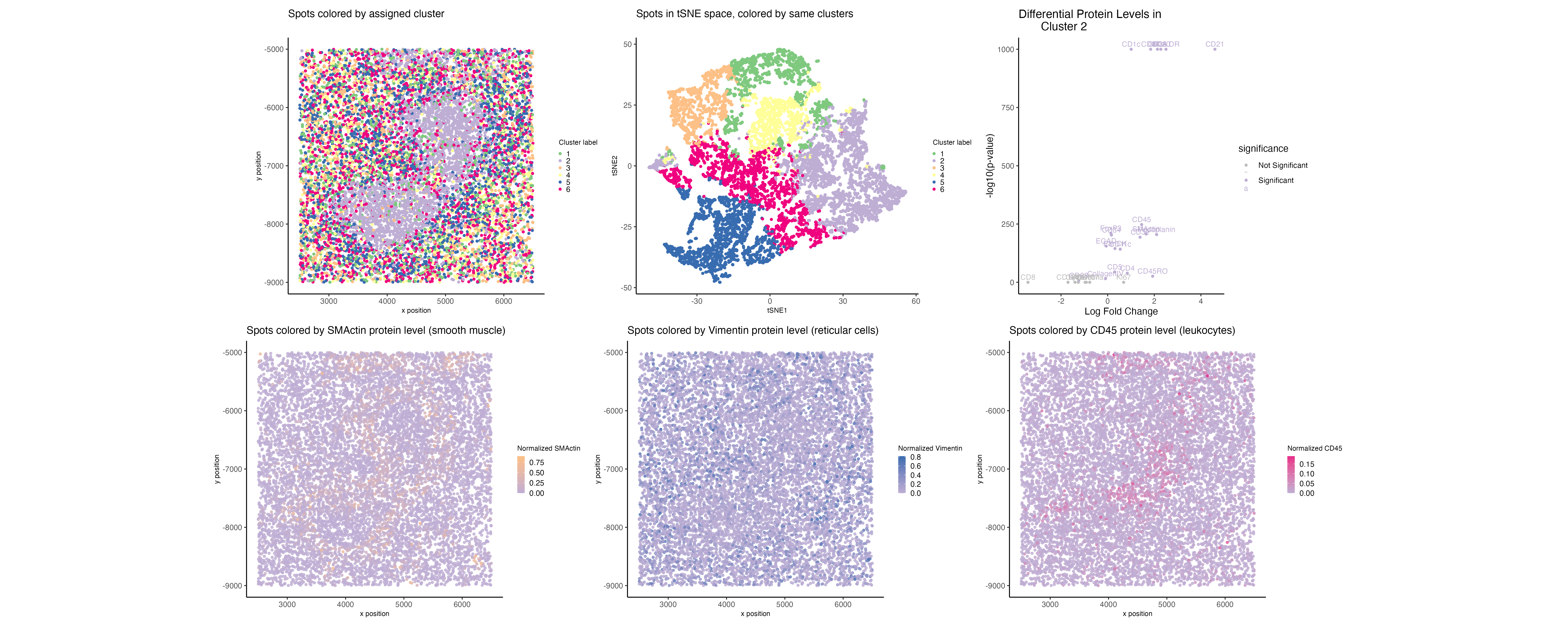
I just started by looking at the overall highest detected proteins and noticed many markers of immune cells, as well as proteins like Vimentin and SMActin (associated with endothelial/fibroblast cells and smooth muscle, respectively) [1,2].
Based on the results of clustering via k-means on the normalized protein levels, there appears to be a clear inner region (shaped a bit like a figure-8) and a surrounding outer region. This is consistent with the anatomy of the spleen, wherein the inner region is the white pulp and the outer region is the red pulp.
I looked at the upregulated proteins in the figure-8 region. One of these was CD45, a marker common to leukocytes and not found on RBCs [3]. This was evidence that this region could be the white pulp. Other upregulated proteins of interest included HLA-DR (expressed by cells like dendritic cells and B cells) [4] and FoxP3 (a regulatory T cell marker) [5].
Importantly, Vimentin was not upregulated in the figure-8 region—this led me to reason that the surrounding structure could comprise many reticular cells, consistent with the red pulp region [6].
I looked at various genes in physical space and was particularly struck by the SMActin expression pattern, which seems to line the figure-8 region. This makes sense to me, given that Pinkus et al. looked at the localization of smooth muscle in the spleen and found a circular/circumferential pattern [7].

References:

https://www.sciencedirect.com/topics/biochemistry-genetics-and-molecular-biology/vimentin#:~:text=Vimentin%20is%20an%20intermediate%20filament%20protein%20found%20in%20many%20types,days%20to%20weeks%20of%20proliferation
https://www.mayocliniclabs.com/test-catalog/overview/70551
https://www.sciencedirect.com/science/article/pii/S0006497120738280#:~:text=THE%20LEUKOCYTE%20COMMON%20antigen%20(CD45)%20is%20an%20abundant%20cell%20surface,10%25%20of%20cell%20membrane%20proteins.&text=It%20is%20a%20member%20of%20the%20protein%20tyrosine%20phosphatase%20family.
https://onlinelibrary.wiley.com/doi/10.1002/pros.20432
https://www.nature.com/articles/nri.2017.75
https://www.sciencedirect.com/topics/medicine-and-dentistry/spleen-cell#:~:text=Besides%20reticular%20cells%2C%20the%20red,nodules%20appended%20to%20the%20sheaths.
https://pmc.ncbi.nlm.nih.gov/articles/PMC1888274/?page=6

Code (paste your code in between the ``` symbols)

library(ggplot2)
library(patchwork)
library(Rtsne)

#### read in data and normalize ####
data <- read.csv('~/Desktop/GDV/genomic-data-visualization-2025/data/codex_spleen_3.csv.gz')
pos <- data[,2:3]
areas <- data[,4]
prots <- data[,5:ncol(data)]
rownames(pos) <- data[,1]
rownames(prots) <- data[,1]

# using library size normalization #
norm_prots <- prots/rowSums(prots)

#### look for overall highest vals, formulate hypotheses ####
tot_prots <- colSums(prots)
names(tot_prots) <- colnames(prots)
tot_prots <- sort(tot_prots)

#### visualize spots and kmeans clusters ####

# kmeans
set.seed(6)
ks <- c(2,3,4,5,6,7,8,9,10,11,12)
totws <- sapply(ks, function(k) {
  print(k)
  clus <- kmeans(norm_prots, centers = k)
  return(clus$tot.withinss)
})

totws_df <- data.frame(k = ks, totw = totws)

# elbow plot
elbow_plt <- ggplot(totws_df, aes(x = k, y = totw)) + 
  geom_point() +
  theme_classic() +
  theme(plot.title = element_text(size = 8), 
        axis.title.x = element_text(size = 8), 
        axis.title.y = element_text(size = 8), 
        legend.title = element_text(size = 8)) +
  labs(x = 'k', y = 'Total Withiness', 
       title = 'Elbow plot for determining # of clusters')

print(elbow_plt)

# using labels w/ 8 clusters 
clus_labs <- (kmeans(norm_prots, centers = 8))$cluster
clus_labs <- as.factor(clus_labs)

# plotting spots in physical space, colored by cluster
clus_in_space <- ggplot(pos, aes(x = x, y = y, 
                                 color = clus_labs)) + 
  geom_point(size = 1) + 
  theme_classic() +
  theme(plot.title = element_text(size = 8), 
        axis.title.x = element_text(size = 8), 
        axis.title.y = element_text(size = 8), 
        legend.title = element_text(size = 8), 
        legend.key.size = unit(0.1,'cm')) +
  scale_color_brewer(palette="Dark2") + 
  labs(x = 'x position', y = 'y position', 
       title = 'Spots colored by assigned cluster', color = 'Cluster label') 

print(clus_in_space)

#### diff gexp analysis ####

# clusters of interest
ct6 <- names(clus_labs)[which(clus_labs == 6)]
ct6other <- names(clus_labs)[which(clus_labs != 6)]

ct5 <- names(clus_labs)[which(clus_labs == 5)]
ct5other <- names(clus_labs)[which(clus_labs != 5)]

ct1 <- names(clus_labs)[which(clus_labs == 1)]
ct1other <- names(clus_labs)[which(clus_labs != 1)]

# wilcox one-sided tests for clusters of interest
results6 <- sapply(colnames(norm_prots), function(i) {
  wilcox.test(norm_prots[ct6, i], norm_prots[ct6other, i], 
              alternative = 'greater')$p.value ## two sided test
})
names(results6) <- colnames(norm_prots)
results6 <- sort(results6)

results5 <- sapply(colnames(norm_prots), function(i) {
  wilcox.test(norm_prots[ct5, i], norm_prots[ct5other, i], 
              alternative = 'greater')$p.value ## two sided test
})
names(results5) <- colnames(norm_prots)
results5 <- sort(results5)

results1 <- sapply(colnames(norm_prots), function(i) {
  wilcox.test(norm_prots[ct1, i], norm_prots[ct1other, i], 
              alternative = 'greater')$p.value ## two sided test
})
names(results1) <- colnames(norm_prots)
results1 <- sort(results1)

#### using fewer clusters ####

# using labels w/ 6 clusters 
set.seed(10)
clus_labs_2 <- (kmeans(norm_prots, centers = 6))$cluster
clus_labs_2 <- as.factor(clus_labs_2)

# plotting spots in physical space, colored by cluster
clus_in_space_2 <- ggplot(pos, aes(x = x, y = y, 
                                 color = clus_labs_2)) + 
  geom_point(size = 1) + 
  theme_classic() +
  theme(plot.title = element_text(size = 12), 
        axis.title.x = element_text(size = 8), 
        axis.title.y = element_text(size = 8), 
        legend.title = element_text(size = 8), 
        legend.key.size = unit(0.1,'cm')) +
  scale_color_brewer(palette="Accent") + 
  labs(x = 'x position', y = 'y position', 
       title = 'Spots colored by assigned cluster', color = 'Cluster label') 

print(clus_in_space_2)

#### visualize clusters in PC space ####

# plotting spots in PC space, colored by cluster
pcs <- prcomp(norm_prots)
pcs_df <- data.frame(pcs$x) 

clus_in_PC_space <- ggplot(pcs_df, aes(x = PC1, y = PC2, 
                                       color = as.factor(clus_labs_2))) + 
  geom_point(size = 2) + 
  theme_classic() +
  theme(plot.title = element_text(size = 8), 
        axis.title.x = element_text(size = 8), 
        axis.title.y = element_text(size = 8), 
        legend.title = element_text(size = 8), 
        legend.key.size = unit(0.1,'cm')) +
  scale_color_brewer(palette="Accent") + 
  labs(title = 'Spots in PC space, colored by same clusters', 
       color = 'Cluster label')

print(clus_in_PC_space)

#### visualize clusters in tSNE space ####

emb <- Rtsne(norm_prots)

tsne_df <- data.frame(tSNE1 = emb$Y[,1], tSNE2 = emb$Y[,2])
tsne_plt <- ggplot(tsne_df, aes(x = tSNE1, y = tSNE2, 
                                color = as.factor(clus_labs_2))) + 
  geom_point(size = 1) + 
  theme_classic() +
  theme(plot.title = element_text(size = 12), 
        axis.title.x = element_text(size = 8), 
        axis.title.y = element_text(size = 8), 
        legend.title = element_text(size = 8), 
        legend.key.size = unit(0.1,'cm')) +
  scale_color_brewer(palette="Accent") + 
  labs(title = 'Spots in tSNE space, colored by same clusters', 
       color = 'Cluster label')

#### diff gexp analysis w/ new clusters ####

ct1_new <- names(clus_labs_2)[which(clus_labs_2 == 2)]
ct1other_new <- names(clus_labs_2)[which(clus_labs_2 != 2)]

results1_new <- sapply(colnames(norm_prots), function(i) {
  wilcox.test(norm_prots[ct1_new, i], norm_prots[ct1other_new, i], 
              alternative = 'greater')$p.value ## two sided test
})
names(results1_new) <- colnames(norm_prots)
results1_new <- data.frame(results1_new)
colnames(results1_new) <- 'results'

# plot volcano plt

mean_prots_ct1 <- colMeans(norm_prots[ct1_new, ])
mean_prots_other <- colMeans(norm_prots[ct1other_new, ])

logFC <- log2(mean_prots_ct1/mean_prots_other)

volcano_df <- data.frame(protein = names(logFC), 
                         logFC = logFC, 
                         p_val = results1_new$results)

volcano_df$pval_log <- -log10(volcano_df$p_val)
volcano_df$pval_log[is.infinite(volcano_df$pval_log)] <- 1000
volcano_df$significance <- ifelse(volcano_df$p_val < 0.01, 
                                  "Significant", "Not Significant")

volcano_plt <- ggplot(volcano_df, aes(x = logFC, y = pval_log, 
                                      color = significance, 
                                      label = protein)) + 
  geom_point(size = 1) + 
  geom_text(vjust = -0.5, size = 3) +
  scale_color_manual(values = c("Significant" = "#beaed4", 
                                "Not Significant" = "grey")) +
  theme(plot.title = element_text(size = 6), 
        axis.title.x = element_text(size = 6), 
        axis.title.y = element_text(size = 6), 
        legend.title = element_text(size = 6)) +
  theme_classic() +
  labs(title = "Differential Protein Levels in 
       Cluster 2", x = "Log Fold Change", 
       y = "-log10(p-value)")

#### visualize cell types ####

CD45_cells <- ggplot(pos, aes(x = x, y = y, 
                               color = norm_prots$CD45)) + 
  geom_point(size = 1, alpha = 0.8) + 
  theme_classic() +
  theme(plot.title = element_text(size = 12), 
        axis.title.x = element_text(size = 8), 
        axis.title.y = element_text(size = 8), 
        legend.title = element_text(size = 8), 
        legend.key.size = unit(0.3,'cm')) +
  scale_color_gradient(low = '#beaed4', high = '#e7298a') + 
  labs(x = 'x position', y = 'y position', 
       title = 'Spots colored by CD45 protein level (leukocytes)', 
       color = 'Normalized CD45')

vimentin_cells <- ggplot(pos, aes(x = x, y = y, 
                              color = norm_prots$Vimentin)) + 
  geom_point(size = 1, alpha = 0.8) + 
  theme_classic() +
  theme(plot.title = element_text(size = 12), 
        axis.title.x = element_text(size = 8), 
        axis.title.y = element_text(size = 8), 
        legend.title = element_text(size = 8), 
        legend.key.size = unit(0.3,'cm')) +
  scale_color_gradient(low = '#beaed4', high = '#386cb0') + 
  labs(x = 'x position', y = 'y position', 
       title = 'Spots colored by Vimentin protein level (reticular cells)', 
       color = 'Normalized Vimentin')

SMA_cells <- ggplot(pos, aes(x = x, y = y, 
                                  color = norm_prots$SMActin)) + 
  geom_point(size = 1, alpha = 0.8) + 
  theme_classic() +
  theme(plot.title = element_text(size = 12), 
        axis.title.x = element_text(size = 8), 
        axis.title.y = element_text(size = 8), 
        legend.title = element_text(size = 8), 
        legend.key.size = unit(0.3,'cm')) +
  scale_color_gradient(low = '#beaed4', high = '#fdc086') + 
  labs(x = 'x position', y = 'y position', 
       title = 'Spots colored by SMActin protein level (smooth muscle)', 
       color = 'Normalized SMActin')

#### final plot ####

clus_in_space_2 <- clus_in_space_2 + coord_fixed(ratio = 1)
tsne_plt <- tsne_plt + coord_fixed(ratio = 1)
volcano_plt <- volcano_plt + coord_fixed(ratio = 0.01)
SMA_cells <- SMA_cells + coord_fixed(ratio = 1)
vimentin_cells <- vimentin_cells + coord_fixed(ratio = 1)
CD45_cells <- CD45_cells + coord_fixed(ratio = 1)

plot <- (clus_in_space_2 + tsne_plt + volcano_plt) / 
  (SMA_cells + vimentin_cells + CD45_cells)

ggsave("~/Desktop/hw5_srahma22.png", plot, width = 25, height = 10, dpi = 300)

27 Feb 2025

« Analyzing Immune Cell Clusters in CODEX Dataset Identifying White Pulp Tissue Structure in CODEX Data »