B and T cells in spleen data

Description
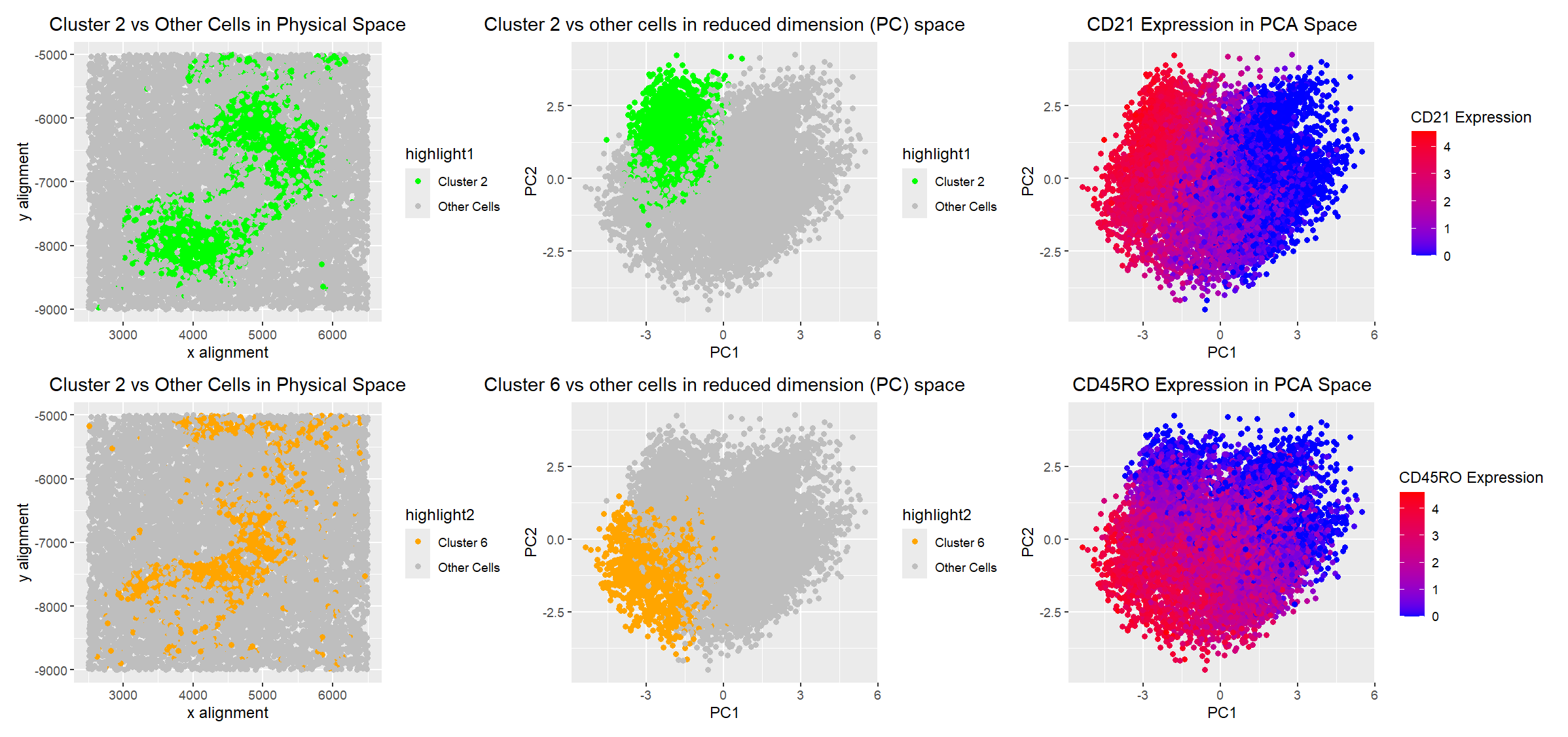
After clustering my data, I visualized two groups of cells. One was centered in physical space, and the other appeared to surround the centered cluster. I began with the ‘surrounding’ cluster, which was Cluster 2 of 6 in my dataset (the number was chosen based on the plot of total weights). The main differentially expressed gene in cluster 2 was CD21, which is mostly expressed in B cells [1]. The main differentially expressed gene in cluster 6 was CD45RO, which is mostly expressed in T cells [2]. The portion of the spleen that contains B and T cells is the white pulp, so I believe this is what the CODEX data was displaying [3]. Additionally, it is common for white pulp to have T cell zones [3], which I believe is why my cluster 6 was in a circle surrounded by non-T cells, whereas some of the other clusters were more spread out.
- https://www.sciencedirect.com/science/article/abs/pii/S1567576900000461
- https://www.sciencedirect.com/topics/immunology-and-microbiology/cd45ro-antigen
- https://www.sciencedirect.com/topics/immunology-and-microbiology/cd45ro-antigen
Code
1
2
3
4
5
6
7
8
9
10
11
12
13
14
15
16
17
18
19
20
21
22
23
24
25
26
27
28
29
30
31
32
33
34
35
36
37
38
39
40
41
42
43
44
45
46
47
48
49
50
51
52
53
54
55
56
57
58
59
60
61
62
63
64
65
66
67
68
69
70
71
72
73
74
75
76
77
78
79
80
81
82
83
84
85
86
87
88
89
90
91
92
93
94
95
96
97
98
99
100
101
102
103
104
105
106
107
108
109
110
111
112
113
114
115
116
117
118
119
120
121
122
123
124
125
126
127
128
129
130
131
132
133
134
135
136
137
138
139
140
141
142
143
144
145
146
147
148
149
150
151
152
153
154
155
156
157
158
159
160
161
162
163
164
165
166
167
168
169
170
171
172
173
174
175
176
177
178
179
180
181
182
183
184
185
186
187
188
189
190
191

library(ggplot2)
library(patchwork)

file <- "data/codex_spleen_3.csv.gz"
data <- read.csv(file)
data[1:5,1:10]

pos <- data[, 3:4]
rownames(pos) <- data$cell_id
gexp <- data[, 5:ncol(data)]
rownames(gexp) <- data$barcode

## if you normalize, if you log transform
## you can use different transformations of the gene expression
## for different parts of the analysis
loggexp <- log10(gexp+1)

ks = 1:30
totw <- sapply(ks, function(k) {
  print(k)
  com <- kmeans(gexp, centers=k)
  return(com$tot.withinss)
})
## how can I use this information?
plot(ks, totw) ## change this to ggplot

#Set seed for reproducability with chosen cluster
set.seed(42)
com <- kmeans(loggexp, centers=6)
clusters <- com$cluster
clusters <- as.factor(clusters) ## tell R it's a categorical variable
names(clusters) <- rownames(gexp)
head(clusters)

pcs <- prcomp(loggexp)
df <- data.frame(pcs$x, clusters)
data$PC1 <- pcs$x[,1]
data$PC2 <- pcs$x[,2]

#using this to pick my cluster of interest
ggplot(data) +
  geom_point(aes(x = x, y=y, col=clusters)) +
  ggtitle("clusters in real space") +
  theme(plot.title = element_text(hjust=0.5)) +
  xlab("x alignment") + ylab("y alignment")

#clusters 2 and 6 have the most speificity in terms of physical space
#so I will look into those
#start with cluster 2
interest <- 2
cellsOfInterest <- names(clusters)[clusters == interest]
otherCells <- names(clusters)[clusters != interest]

# Create a new column for coloring
data$highlight1 <- ifelse(clusters == interest, "Cluster 2", "Other Cells")

p1 <- ggplot(data) +
  geom_point(aes(x = PC1, y = PC2, col = highlight1)) +
  ggtitle("Cluster 2 vs other cells in reduced dimension (PC) space") +
  theme(plot.title = element_text(hjust = 0.5)) +
  xlab("PC1") +
  ylab("PC2") +
  scale_color_manual(values = c("Cluster 2" = "green", "Other Cells" = "gray"))

p2 <- ggplot(data) +
  geom_point(aes(x = x, y = y, col = highlight1)) +
  ggtitle("Cluster 2 vs Other Cells in Physical Space") +
  theme(plot.title = element_text(hjust = 0.5)) +
  xlab("x alignment") +
  ylab("y alignment") +
  scale_color_manual(values = c("Cluster 2" = "green", "Other Cells" = "gray"))

#Differential gene expression
gexp_cluster2 <- loggexp[cellsOfInterest, ]  # Expression in Cluster 2
gexp_other <- loggexp[otherCells, ]          # Expression in other clusters

pvals <- sapply(1:ncol(loggexp), function(i) {
  wilcox.test(gexp_cluster2[, i], gexp_other[, i], exact = FALSE)$p.value
})

#correction as mentioned in class (i picked bonferroni)
adj_pvals <- p.adjust(pvals, method = "bonferroni")

#mean expression diff
logFC <- colMeans(gexp_cluster2) - colMeans(gexp_other)

# Create a dataframe of results
DE_genes <- data.frame(Gene = colnames(loggexp),
                       logFC = logFC, pval = pvals, adj_pval = adj_pvals)

# Filter p-value < 0.05)
DE_genes <- DE_genes[DE_genes$adj_pval < 0.05, ]

# Sort by mean expression diff
DE_genes <- DE_genes[order(DE_genes$logFC, decreasing = TRUE), ]

# Select the top 5 most differentially expressed genes
top5_genes <- DE_genes$Gene[1:5]
print(top5_genes)

# Extract top (CD21) expression across all cells
cd21_expression <- loggexp[, "CD21"]

# Add CD21 expression to the original data
data$cd21_expression <- cd21_expression

p3 <- ggplot(data, aes(x = PC1, y = PC2, color = cd21_expression)) +
  geom_point() +
  scale_color_gradient(low = "blue", high = "red") +
  ggtitle("CD21 Expression in PCA Space") +
  theme(plot.title = element_text(hjust = 0.5)) +
  xlab("PC1") +
  ylab("PC2") +
  labs(color = "CD21 Expression")

#Repeat process for cluster 6
interest <- 6
cellsOfInterest <- names(clusters)[clusters == interest]
otherCells <- names(clusters)[clusters != interest]

# Create a new column for coloring
data$highlight2 <- ifelse(clusters == interest, "Cluster 6", "Other Cells")

p4 <- ggplot(data) +
  geom_point(aes(x = PC1, y = PC2, col = highlight2)) +
  ggtitle("Cluster 6 vs other cells in reduced dimension (PC) space") +
  theme(plot.title = element_text(hjust = 0.5)) +
  xlab("PC1") +
  ylab("PC2") +
  scale_color_manual(values = c("Cluster 6" = "orange", "Other Cells" = "gray"))

p5 <- ggplot(data) +
  geom_point(aes(x = x, y = y, col = highlight2)) +
  ggtitle("Cluster 2 vs Other Cells in Physical Space") +
  theme(plot.title = element_text(hjust = 0.5)) +
  xlab("x alignment") +
  ylab("y alignment") +
  scale_color_manual(values = c("Cluster 6" = "orange", "Other Cells" = "gray"))

#Differential gene expression
gexp_cluster6 <- loggexp[cellsOfInterest, ]  # Expression in Cluster 6
gexp_other <- loggexp[otherCells, ]          # Expression in other clusters

pvals <- sapply(1:ncol(loggexp), function(i) {
  wilcox.test(gexp_cluster2[, i], gexp_other[, i], exact = FALSE)$p.value
})

#correction as mentioned in class (i picked bonferroni)
adj_pvals <- p.adjust(pvals, method = "bonferroni")

#mean expression diff
logFC <- colMeans(gexp_cluster6) - colMeans(gexp_other)

# Create a dataframe of results
DE_genes <- data.frame(Gene = colnames(loggexp),
                       logFC = logFC, pval = pvals, adj_pval = adj_pvals)

# Filter p-value < 0.05)
DE_genes <- DE_genes[DE_genes$adj_pval < 0.05, ]

# Sort by mean expression diff
DE_genes <- DE_genes[order(DE_genes$logFC, decreasing = TRUE), ]

# Select the top 5 most differentially expressed genes
top5_genes <- DE_genes$Gene[1:5]
print(top5_genes)

# Extract top (CD45RO) expression across all cells
cd45_expression <- loggexp[, "CD45RO"]

# Add CD21 expression to the original data
data$cd45_expression <- cd45_expression

p6 <- ggplot(data, aes(x = PC1, y = PC2, color = cd45_expression)) +
  geom_point() +
  scale_color_gradient(low = "blue", high = "red") +
  ggtitle("CD45RO Expression in PCA Space") +
  theme(plot.title = element_text(hjust = 0.5)) +
  xlab("PC1") +
  ylab("PC2") +
  labs(color = "CD45RO Expression")


combined_plot <- (p2 | p1 | p3) / (p5 | p4 | p6)

# Display the combined plot
combined_plot