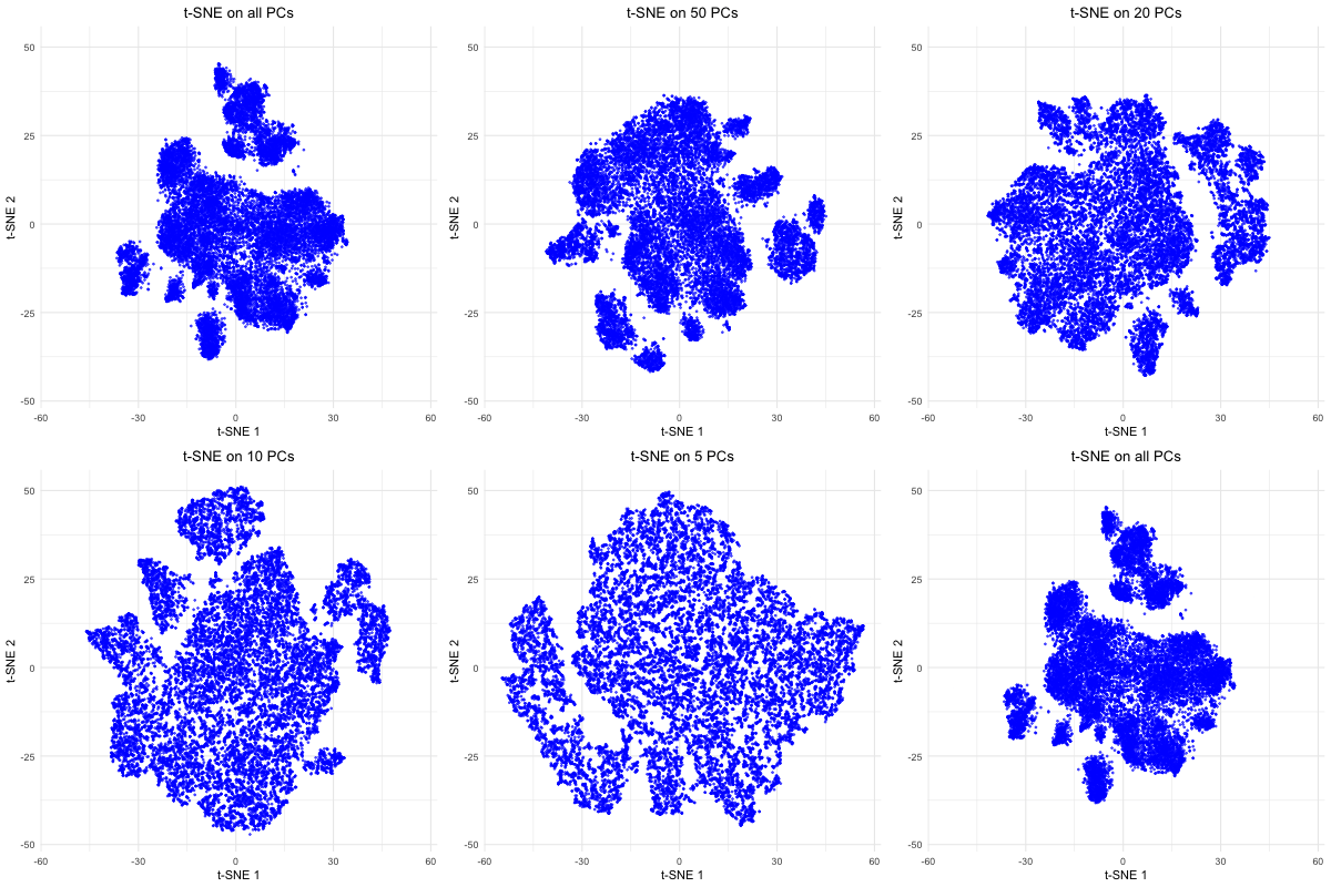
Visualization of t-SNE on Different PC Counts on Pikachu Dataset

1.If I perform non-linear dimensionality reduction on PCs, what happens when I vary how many PCs should I use?
The figure visualizes how varying the number of principal components (PCs) affects t-SNE embeddings of smFISH Pikachu dataset. The animation cycles through t-SNE results computed with 5, 10, 20, 50, and all PCs, showing how the structure of the reduced 2D space changes as more variance is included. With only a few PCs, the embedding lacks clear structure. As more PCs are incorporated (20–50), the separation of clusters becomes more distinct. However, when all PCs are included, the embedding appears noisier, likely due to the inclusion of low-variance PCs. This demonstrates that selecting an optimal number of PCs helps capture variation in the spatial transcriptomics data while avoiding unnecessary complexity, which allows better t-SNE visualizations.
5. Code
1
2
3
4
5
6
7
8
9
10
11
12
13
14
15
16
17
18
19
20
21
22
23
24
25
26
27
28
29
30
31
32
33
34
35
36
37
38
39
40
41
42
43
44
45
46
47
48
49
50
51
52
53
## libraries
library(gganimate)
library(ggplot2)
library(Rtsne)
library(dplyr)
library(viridis)

# Read data
file <- '~/Desktop/genomic-data-visualization-2025/data/pikachu.csv.gz'
data <- read.csv(file)

# Extract gene expression data
gexp <- data[, 7:ncol(data)]
rownames(gexp) <- data$barcode

# Normalize data by total gene expression per cell
gexp_norm <- gexp / rowSums(gexp)

# Perform PCA
pcs <- prcomp(gexp_norm, center = TRUE, scale. = FALSE)

# Perform t-SNE
set.seed(42)
tsne_5 <- Rtsne(pcs$x[, 1:5], dims = 2, pca = FALSE)
tsne_10 <- Rtsne(pcs$x[, 1:10], dims = 2, pca = FALSE)
tsne_20 <- Rtsne(pcs$x[, 1:20], dims = 2, pca = FALSE)
tsne_50 <- Rtsne(pcs$x[, 1:50], dims = 2, pca = FALSE)
tsne_all <- Rtsne(pcs$x, dims = 2, pca = FALSE)

# data frame
plot.df <- bind_rows(
  data.frame(tsne_x = tsne_5$Y[,1], tsne_y = tsne_5$Y[,2], order = "t-SNE on 5 PCs"),
  data.frame(tsne_x = tsne_10$Y[,1], tsne_y = tsne_10$Y[,2], order = "t-SNE on 10 PCs"),
  data.frame(tsne_x = tsne_20$Y[,1], tsne_y = tsne_20$Y[,2], order = "t-SNE on 20 PCs"),
  data.frame(tsne_x = tsne_50$Y[,1], tsne_y = tsne_50$Y[,2], order = "t-SNE on 50 PCs"),
  data.frame(tsne_x = tsne_all$Y[,1], tsne_y = tsne_all$Y[,2], order = "t-SNE on all PCs")
) %>% mutate(order = factor(order, levels = rev(unique(order))))

# Create animation plot
p <- ggplot(plot.df, aes(x = tsne_x, y = tsne_y)) +
  geom_point(size = 0.5, alpha = 0.6, color = "blue") +
  theme_minimal() +
  labs(x = "t-SNE 1", y = "t-SNE 2", title = '{closest_state}') +
  theme(plot.title = element_text(hjust = 0.5)) +
  transition_states(order, transition_length = 2, state_length = 1) +
  ease_aes('cubic-in-out')

# Render and store animation
anim_obj <- animate(p, height = 400, width = 400, fps = 5, renderer = gifski_renderer())

# Save animation
save("hwEC1_knguye72.gif", animation = anim_obj)
