Kidney PCA vs Loading Size Analysis(Prompt 2)

1. What data types are you visualizing?
Cell identification is categorical/nominal, in that it is number and letter labeled bins/categories in which I am counting gene expression. There is spatial data in the physical location of the cell in the x and y coordinates. There is quantitative data, representing how much of a gene is expressed in each cell, though in this case we are looking at both this for the spatial mapping, and the number of genes per loading bin. The loading bin labels are a form of ordinal data. The mapping is a form of relational data.
2. What data encodings (geometric primitives and visual channels) are you using to visualize these data types?
I am using points/areas as geometric principles for the spatial mapping, and areas/lines for the histogram, as geometric principles. The size of the area in the histogram represents the number of genes that fall into that bin. The color hue(red vs blue) in the spatial graph helps to differentiate between the identified highest positive and highest negative loading genes, the opacity is by default low meaning clusters overlap and have higher opacity, making it a tool to express expression density in certain locations, and their spatial position helps to differentiate them. The spatial data also reveals the actual structure of the organ cross section. There is low opacity grey hue used to represent any position where the genes aren’t expressed in the spatial map, though it rarely appears due to broad expression of these genes throughout the kidney.
3. What about the data are you trying to make salient through this data visualization?
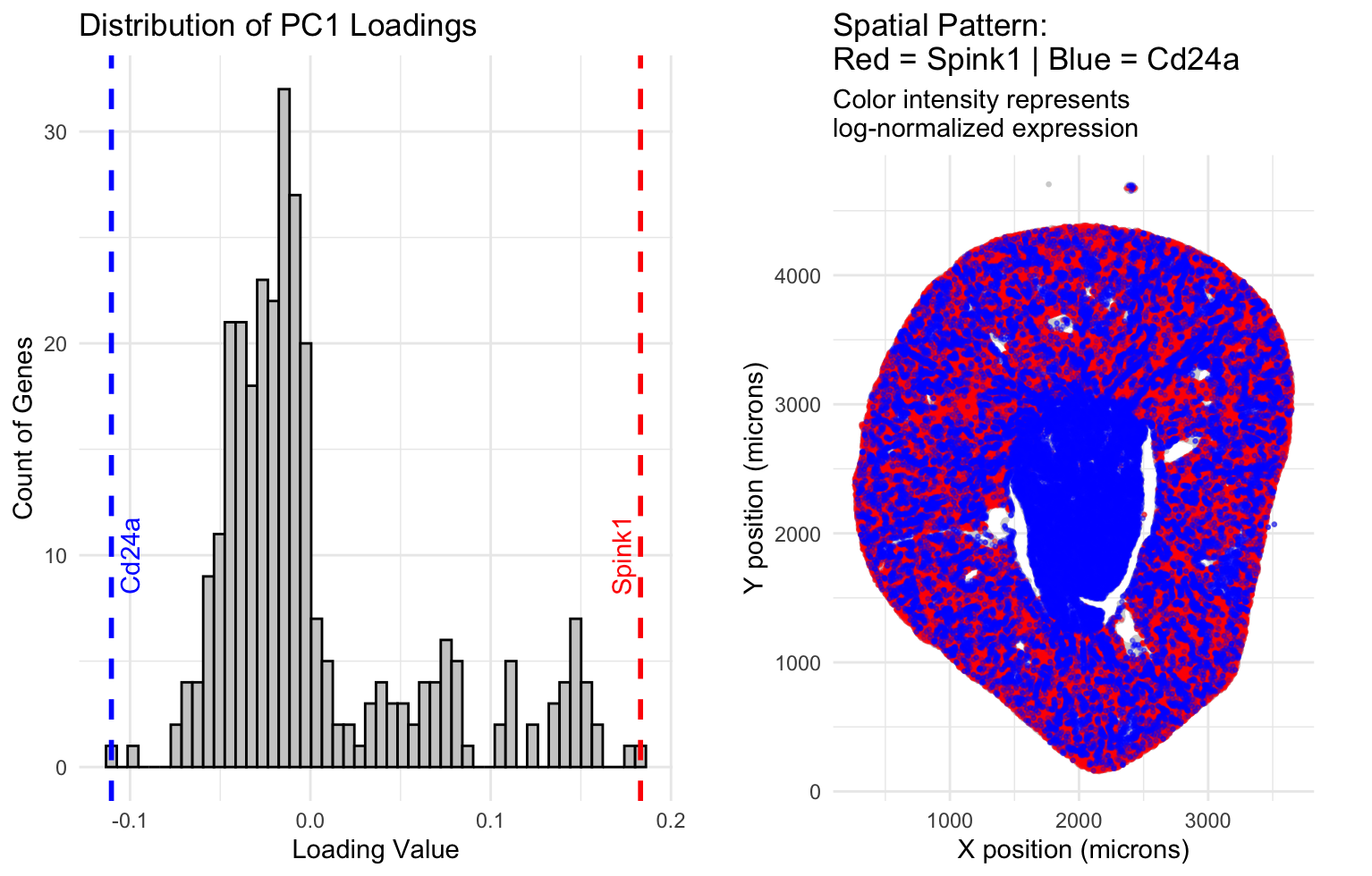
The data visualization seeks to explore the relationship between the gene with the highest positive loading and the gene with the highest negative loading that PC1 has identified. These genes are first characterized on a histogram that makes salient their frequency compared to other loadings. These genes are then mapped onto a spatial graph that uses their position and assigned color in order to make salient where each graph lies relative to the spatial structure of the kidney cross section. The data shows that PC1 has differentiated these two genes by their spatial position, specifically the outer area of the kidney(cortex) is where the highest positive loading gene, Spink1, is most expressed, and the inner area of the kidney(medulla) is where the highest negative loading gene,Cd24a, is most expressed.
4. What Gestalt principles or knowledge about perceptiveness of visual encodings are you using to accomplish this?
Similarity of color and proximity of same color mapping is used to identify clusters of gene expression locations on the spatial map in order to identify what structural principle PC1 identified. Color/continuity(of the dashes) is used in the dashed line on the histogram in order to identify where the identified highest positive and negative loading genes lie relative to the other frequency tallies.
5. Code (paste your code in between the ``` symbols)
1
2
3
4
5
6
7
8
9
10
11
12
13
14
15
16
17
18
19
20
21
22
23
24
25
26
27
28
29
30
31
32
33
34
35
36
37
38
39
40
41
42
43
44
45
46
47
48
49
50
51
52
53
54
55
56
57
58
59
60
61
62
63
64
65
66
67
68
69
70
71
72
73
74
75
76
77
78
79
80
81
82
83
84
85
86
87
88
89
90
91
92
93
94
95
96
97
98

#Prompt: Snippet 1, Lets do the data preparation first, log normalization to capture variance, and scaling and library size normalization so that we can accurately do PCA.
# Load necessary libraries
library(dplyr)
library(ggplot2)
library(gridExtra)

# --- STEP 1: LOAD DATA ---
raw_data <- read.csv("Xenium-IRI-ShamR_matrix.csv", row.names = 1)
spatial_coords <- raw_data %>% select(x, y)
gene_counts_raw <- raw_data %>% select(-x, -y)

# --- STEP 2: LIBRARY SIZE NORMALIZATION (Per Cell) ---
total_counts <- rowSums(gene_counts_raw)
gene_counts_norm <- sweep(gene_counts_raw, 1, total_counts + 1e-6, "/") * 10000

# --- STEP 3: LOG-TRANSFORMATION (Per Gene) ---
gene_counts_log <- log1p(gene_counts_norm)

# --- STEP 4: FILTERING ZERO-VARIANCE GENES ---
sds <- apply(gene_counts_log, 2, sd)
variable_genes_log <- gene_counts_log[, sds > 0]

# --- STEP 5: SCALING (Per Gene) ---
gene_counts_scaled <- scale(variable_genes_log)


#Prompt: Snippet 2, run the PCA. We are going to look for the the genes that have the highest positive and highest negative loading.

# --- STEP 6: PERFORM PCA ---
pca_result <- prcomp(gene_counts_scaled, center = FALSE, scale. = FALSE)

# --- STEP 7: EXTRACT LOADINGS ---
pc1_loadings <- pca_result$rotation[, 1]
sorted_loadings <- sort(pc1_loadings)

# --- STEP 8: SELECT GENES OF INTEREST---
# 1. High Positive Loading (Max value)
gene_high_pos <- names(sort(pc1_loadings, decreasing = TRUE))[1]
val_high_pos <- max(pc1_loadings)

# 2. High Negative Loading (Min value)
gene_high_neg <- names(sort(pc1_loadings, decreasing = FALSE))[1]
val_high_neg <- min(pc1_loadings)

print(paste("High Positive Gene:", gene_high_pos))
print(paste("High Negative Gene:", gene_high_neg))


#Prompt: snippet 3, create the following plots: histogram for loading sizes, taking into account negative and positive. We use a histogram and binning so we aren't just mapping 300 genes on the x axis. Label where the highest and lowest(most negative) genes lie, respectively, then we will have a spatial map of two low ish opacity colors for the top genes per category identified(high pos, high neg), with opacity tracking overlap, and we will have a grey map for the rest of the spatial positions in order to improve saliency for what we are tracking.
# --- STEP 9: PREPARE PLOTTING DATA ---
plot_data <- data.frame(
  x = spatial_coords$x,
  y = spatial_coords$y,
  Pos_Expr = gene_counts_log[, gene_high_pos],
  Neg_Expr = gene_counts_log[, gene_high_neg]
)

# --- STEP 10: PANEL 1 - HISTOGRAM OF LOADINGS ---
loadings_df <- data.frame(gene = names(pc1_loadings), loading = pc1_loadings)

p1 <- ggplot(loadings_df, aes(x = loading)) +
  geom_histogram(bins = 50, fill = "gray80", color = "black") +
  # Mark the High Positive Gene (Red)
  geom_vline(xintercept = val_high_pos, color = "red", linetype = "dashed", size = 1) +
  annotate("text", x = val_high_pos, y = 10, label = gene_high_pos, color = "red", angle = 90, vjust = -0.5) +
  # Mark the High Negative Gene (Blue)
  geom_vline(xintercept = val_high_neg, color = "blue", linetype = "dashed", size = 1) +
  annotate("text", x = val_high_neg, y = 10, label = gene_high_neg, color = "blue", angle = 90, vjust = 1.5) +
  theme_minimal() +
  labs(title = "Distribution of PC1 Loadings", x = "Loading Value", y = "Count of Genes")

# --- STEP 11: PANEL 2 - SPATIAL MAP ---
p2 <- ggplot() +
  # Layer 1: Background Tissue (Grey)
  geom_point(data = plot_data, aes(x = x, y = y), color = "lightgrey", size = 0.5) +

  # Layer 2: High Positive Gene (Red)
  geom_point(data = subset(plot_data, Pos_Expr > 0),
             aes(x = x, y = y, alpha = Pos_Expr), color = "red", size = 0.5) +

  # Layer 3: High Negative Gene (Blue)
  geom_point(data = subset(plot_data, Neg_Expr > 0),
             aes(x = x, y = y, alpha = Neg_Expr), color = "blue", size = 0.5) +

  scale_alpha_continuous(range = c(0.1, 0.8), guide = "none") +
  coord_fixed() +
  theme_minimal() + # Shows the X and Y axes
  labs(
    title = paste("Spatial Pattern:\nRed =", gene_high_pos, "| Blue =", gene_high_neg),
    subtitle = "Color intensity represents\nlog-normalized expression", # \n splits the line
    x = "X position (microns)",
    y = "Y position (microns)"
  )
# --- STEP 12: COMBINE AND DISPLAY ---
grid.arrange(p1, p2, ncol = 2)