Identification and Characterization of a Transcriptionally Distinct Endothelial-Like Cluster in Xenium Kidney Spatial Transcriptomics Data

1. Describe your figure briefly.
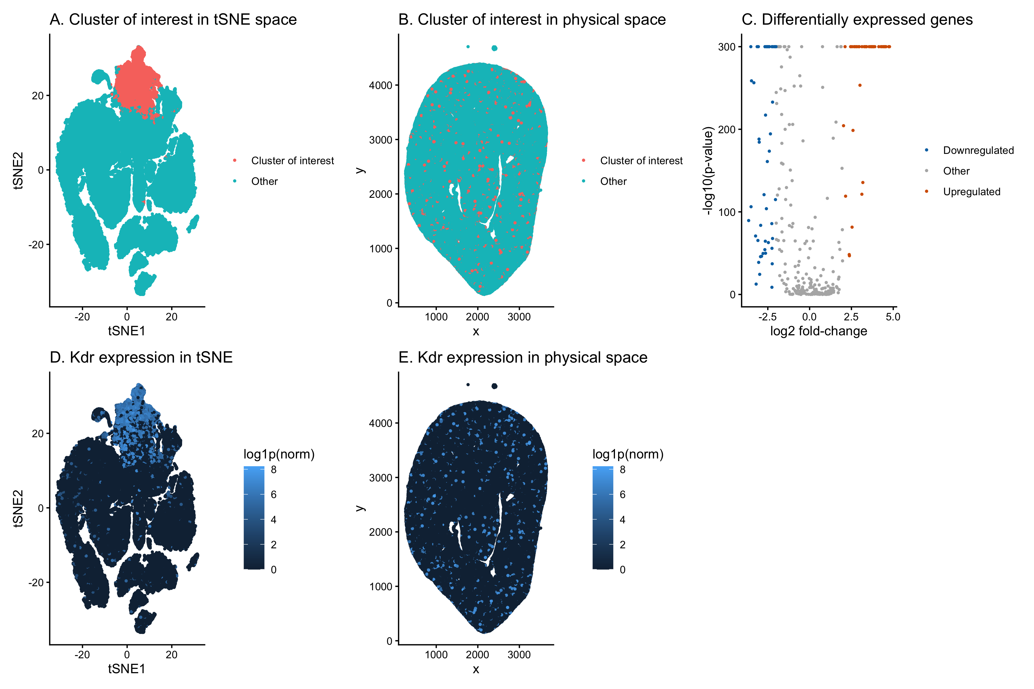
In these panels, I depict the representation of the Xenium kidney spatial transcriptomics dataset in latent tSNE-embedded space and over the original spatial slide coordinates. Prior to clustering, I evaluated a range of k values (k = 2–20) using k-means clustering on the first 15 principal components and assessed the total within-cluster sum of squares to identify an elbow point. Based on this analysis, I selected k = 10 as a balance between capturing transcriptional heterogeneity and avoiding over-fragmentation of clusters.
Using k = 10, I examined the resulting clusters in tSNE-embedded space and identified one cluster that forms a compact and well-separated group relative to surrounding clusters (A). This cluster was selected as the cluster of interest because its clear separation in latent space suggests a transcriptionally distinct population. I then visualized the spatial organization of the same cluster of spots on the spatial array (B).
| Next, I performed a Wilcoxon rank-sum test and computed log2 fold change for each gene in the selected cluster with respect to expression levels of the same genes across all other spots. Differential gene expression is represented as a function of magnitude of differential expression (log2 fold change) and statistical significance (p-value) and is visualized using a volcano plot (C). Genes with p-value < 1e-5 and | log2 fold change | > 2 are considered significantly differentially expressed. |
From this plot, I identify Kdr as a top upregulated gene within the cluster of interest. Kdr is selected because it exhibits strong upregulation and high statistical significance. I then visualize the normalized expression of Kdr across the tSNE-embedded space and over the original spatial coordinates (D, E). Elevated Kdr expression is concentrated within the selected cluster in tSNE space and broadly distributed throughout the tissue in physical space, consistent with the widespread vascular network in kidney tissue. Importantly, prior studies have established Kdr (also known as VEGFR-2) as a canonical marker of vascular endothelial cells and a principal mediator of VEGF-driven endothelial signaling[1]. Therefore, the strong enrichment of Kdr in this cluster supports the interpretation that the selected cluster likely corresponds to an endothelial-like cell population.
Based on the strong enrichment of Kdr and its known biological function in endothelial cells, I conclude that the selected cluster likely corresponds to an endothelial-like cell population.
[1]Shah FH, Nam YS, Bang JY, Hwang IS, Kim DH, Ki M, Lee HW. Targeting vascular endothelial growth receptor-2 (VEGFR-2): structural biology, functional insights, and therapeutic resistance. Arch Pharm Res. 2025 May;48(5):404-425. doi: 10.1007/s12272-025-01545-1. Epub 2025 May 8. PMID: 40341988; PMCID: PMC12106596.
2. Code (paste your code in between the ``` symbols)
1
2
3
4
5
6
7
8
9
10
11
12
13
14
15
16
17
18
19
20
21
22
23
24
25
26
27
28
29
30
31
32
33
34
35
36
37
38
39
40
41
42
43
44
45
46
47
48
49
50
51
52
53
54
55
56
57
58
59
60
61
62
63
64
65
66
67
68
69
70
71
72
73
74
75
76
77
78
79
80
81
82
83
84
85
86
87
88
89
90
91
92
93
94
95
96
97
98
99
100
101
102
103
104
105
106
107
108
109
110
111
112
113
114
115
116
117
118
119
120
121
122
123
124
125
126
127
128
129
130
131
132
133
134
135
136
137
138
139
140
141
142
143
144
145
146
147
148
149
150
151
152
153
154
155
156
157
158
159
160
161
162
163
164
165
166
167
168
169
170
171
172
173
174
175
176
177
178
179
180
181
182
183
184
185
186
187
188
189
190
191
192
193
194
195
196
197
198
199
200
201
202
203
204
205
206
207
208
209
210
211
212
213
214
215
216
217
218
219
220
221
222
223
224
225
226
227
228
229
230
231
232
233
234
235
236
237
238
239
240
241
242
243
244
245
246
247
## ---------------------------
## 0) Load required packages
## ---------------------------
pkgs <- c("data.table", "ggplot2", "patchwork", "Rtsne")

to_install <- pkgs[!pkgs %in% rownames(installed.packages())]
if (length(to_install) > 0) {
  install.packages(to_install, dependencies = TRUE)
}

library(data.table)
library(ggplot2)
library(patchwork)
library(Rtsne)


set.seed(123)

## ---------------------------
## 1) Load data
## ---------------------------
file <- "/Users/xl/Desktop/JHU2026Spring/Genomic-Data-Visualization/Homework/HW3/Xenium-IRI-ShamR_matrix.csv.gz"
dt <- fread(file)

cat("Data dimensions:", dim(dt), "\n")

## 2) Explicitly set columns
barcode_col <- "V1"
x_col <- "x"
y_col <- "y"

stopifnot(all(c(barcode_col, x_col, y_col) %in% colnames(dt)))

barcodes <- dt[[barcode_col]]

pos <- data.frame(
  aligned_x = dt[[x_col]],
  aligned_y = dt[[y_col]]
)
rownames(pos) <- barcodes

## 3) Expression matrix: all remaining columns are genes
gene_cols <- setdiff(colnames(dt), c(barcode_col, x_col, y_col))

# Convert to numeric matrix safely
gexp_dt <- dt[, ..gene_cols]

for (cc in colnames(gexp_dt)) {
  if (!is.numeric(gexp_dt[[cc]])) {
    gexp_dt[[cc]] <- as.numeric(gexp_dt[[cc]])
  }
}

gexp <- as.matrix(gexp_dt)
rownames(gexp) <- barcodes

# Remove all-zero genes
gexp <- gexp[, colSums(gexp, na.rm = TRUE) > 0, drop = FALSE]

cat("Expression matrix dim:", dim(gexp), "\n")

## 4) Feature selection + normalization
topN <- 1500
gene_order <- order(colSums(gexp), decreasing = TRUE)
head(gene_order)
topgenes <- colnames(gexp)[gene_order[1:min(topN, ncol(gexp))]]
gsub <- gexp[, topgenes, drop = FALSE]

libsize <- rowSums(gsub)
libsize[libsize == 0] <- 1

norm <- (gsub / libsize) * 1e4
logexp <- log1p(norm)

## 5) PCA + kmeans
pcs <- prcomp(logexp, center = TRUE, scale. = TRUE)

ks <- 2:20

totw <- sapply(ks, function(k) {
  km_tmp <- kmeans(pcs$x[,1:15], centers = k, nstart = 20)
  km_tmp$tot.withinss
})

elbow_df <- data.frame(k = ks, tot_withinss = totw)

ggplot(elbow_df, aes(x = k, y = tot_withinss)) +
  geom_point(size = 2) +
  geom_line() +
  labs(title = "Elbow plot for choosing k",
       x = "Number of clusters (k)",
       y = "Total within-cluster sum of squares") +
  theme_classic()

k_final <- 10
km <- kmeans(pcs$x[, 1:15], centers = k_final, nstart = 25)
clusters <- km$cluster

pca_df <- data.frame(
  PC1 = pcs$x[,1],
  PC2 = pcs$x[,2],
  cluster = factor(clusters)
)

ggplot(pca_df, aes(PC1, PC2, color = cluster)) +
  geom_point(size = 0.6) +
  labs(title = "PCA of kidney Xenium data colored by k-means clusters",
       color = "Cluster") +
  theme_classic()

## 6) Pick a cluster of interest
pca_xy <- pcs$x[, 1:2]
interest <- 4
cat("Cluster of interest:", interest, "\n")

cells_interest <- barcodes[clusters == interest]
cells_other <- barcodes[clusters != interest]

## 7) Differential expression (Wilcoxon)
wilcox_p <- sapply(colnames(logexp), function(g) {
  x <- logexp[cells_interest, g]
  y <- logexp[cells_other, g]
  suppressWarnings(wilcox.test(x, y)$p.value)
})


log2fc <- sapply(colnames(norm), function(g) {
  log2((mean(norm[cells_interest, g]) + 1e-3) /
         (mean(norm[cells_other, g]) + 1e-3))
})

de_df <- data.frame(
  gene = names(wilcox_p),
  pval = as.numeric(wilcox_p),
  neglog10p = -log10(as.numeric(wilcox_p) + 1e-300),
  log2fc = as.numeric(log2fc[names(wilcox_p)])
)

de_df <- de_df[order(de_df$pval, -de_df$log2fc), ]


ggplot(de_df, aes(x = log2fc, y = neglog10p)) +
  geom_point(size = 0.6) +
  geom_vline(xintercept = c(-1, 1), linetype = "dashed") +
  geom_hline(yintercept = -log10(1e-5), linetype = "dashed") +
  labs(title = "Volcano plot: cluster of interest vs others",
       x = "log2 fold-change",
       y = "-log10(p-value)") +
  theme_classic()

sig_up <- de_df[de_df$pval < 1e-5 & de_df$log2fc > 1, ]
head(sig_up, 10)


## 8) Choose marker gene
kidney_markers <- c("Lrp2","Slc34a1","Cubn","Aldob",
                    "Slc12a1","Umod","Slc12a3",
                    "Aqp2","Atp6v1b1","Foxi1",
                    "Pecam1","Kdr","Nphs1","Nphs2",
                    "Col1a1","Col3a1","Ptprc","Lyz2",
                    "Aqp1","Aqp4","Aqp6")  #

filtered_de <- de_df[
  de_df$pval < 0.05 & abs(de_df$log2fc) > 1,
]

available <- kidney_markers[kidney_markers %in% filtered_de$gene]

top_markers <- available[
  order(filtered_de$pval[match(available, filtered_de$gene)])
][1:1]

top_markers

marker_gene <- "Kdr"


## 9) tSNE embedding
tsne_res <- Rtsne(pcs$x[, 1:15], perplexity = 30, check_duplicates = FALSE)
emb <- data.frame(tsne_res$Y)
colnames(emb) <- c("tSNE1","tSNE2")
colnames(emb)
head(emb)
emb$is_interest <- ifelse(clusters == interest, "Cluster of interest", "Other")

## 10) Panels
p1 <- ggplot(emb, aes(tSNE1, tSNE2, color = is_interest)) +
  geom_point(size = 0.6) +
  labs(title = "A. Cluster of interest in tSNE space", color = NULL) +
  theme_classic()

sp <- data.frame(pos)
sp$is_interest <- ifelse(clusters == interest, "Cluster of interest", "Other")

p2 <- ggplot(sp, aes(aligned_x, aligned_y, color = is_interest)) +
  geom_point(size = 0.6) +
  labs(title = "B. Cluster of interest in physical space",
       x = "x", y = "y", color = NULL) +
  theme_classic()

de_df$group <- "Other"
de_df$group[de_df$pval < 1e-5 & de_df$log2fc > 2]  <- "Upregulated"
de_df$group[de_df$pval < 1e-5 & de_df$log2fc < -2] <- "Downregulated"

p3 <- ggplot(de_df, aes(log2fc, neglog10p, color = group)) +
  geom_point(size = 0.6) +
  scale_color_manual(
    values = c(
      "Upregulated"   = "#D55E00",   # orange/red
      "Downregulated" = "#0072B2",   # blue
      "Other"         = "grey70"
    )
  ) +
  labs(title = "C. Differentially expressed genes",
       x = "log2 fold-change", y = "-log10(p-value)", color = NULL) +
  theme_classic()

emb$gene_expr <- logexp[, marker_gene]
p4 <- ggplot(emb, aes(tSNE1, tSNE2, color = gene_expr)) +
  geom_point(size = 0.6) +
  labs(title = paste("D.", marker_gene, "expression in tSNE"),
       color = "log1p(norm)") +
  theme_classic()

sp$gene_expr <- logexp[, marker_gene]
p5 <- ggplot(sp, aes(aligned_x, aligned_y, color = gene_expr)) +
  geom_point(size = 0.6) +
  labs(title = paste("E.", marker_gene, "expression in physical space"),
       x = "x", y = "y", color = "log1p(norm)") +
  theme_classic()


multi_panel <- wrap_plots(
  p1, p2, p3,
  p4, p5, plot_spacer(),
  ncol = 3, byrow = TRUE
)

ggsave(
  filename = "multi_panel_cluster_Kdr.png",
  plot = multi_panel,
  width = 12,
  height = 8,
  dpi = 300
)