Identifying a cluster of Proximal Tubule Epithelial Cells

Description
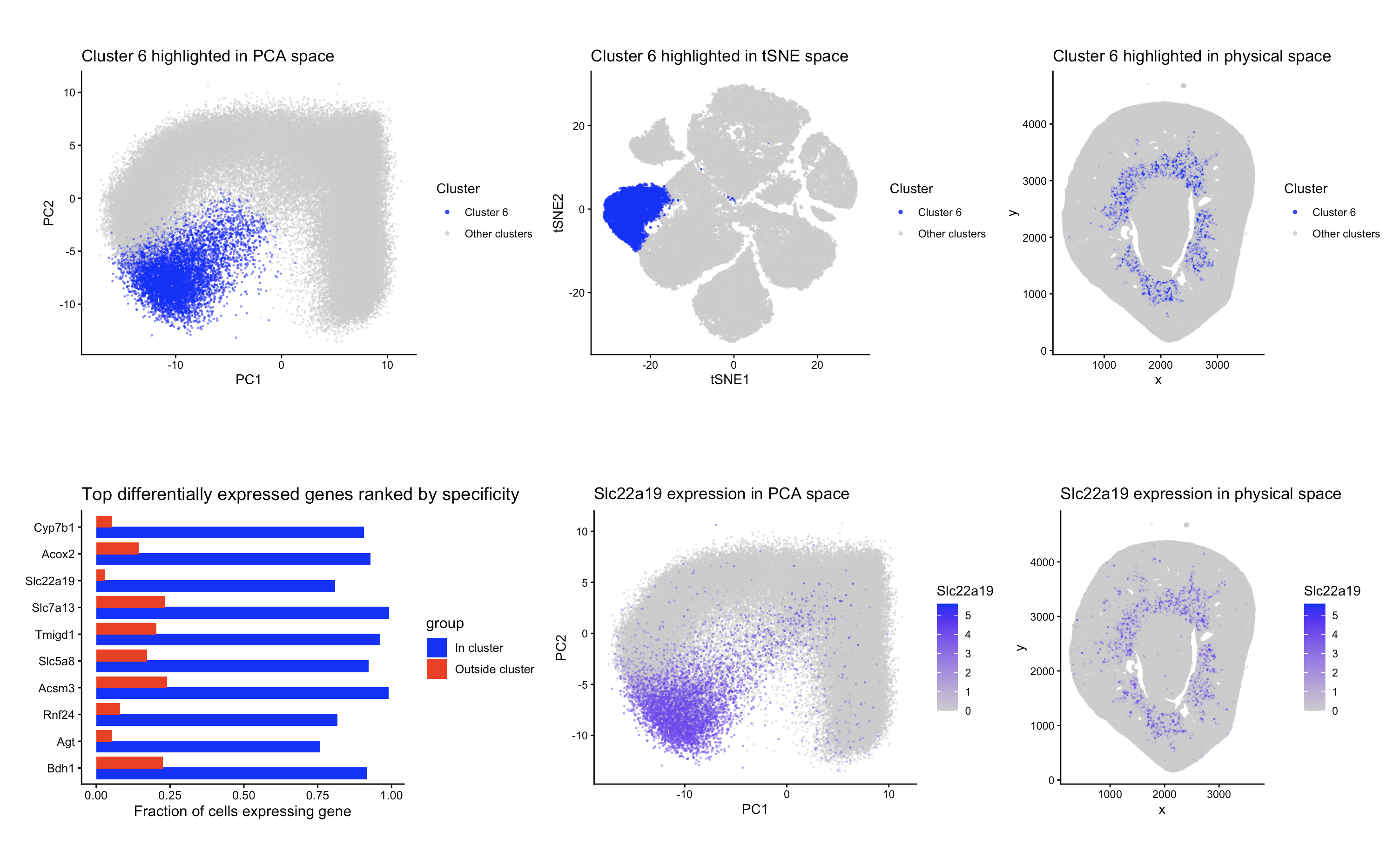
To identify and characterize a transcriptionally distinct cell cluster from the Xenium dataset, I first normalized the raw counts and did PCA for dimensionality reduction. Based on the scree plot I created, I chose to use the first 10 PCs for the rest of my analysis. I then did K-means clustering in the reduced space, and selected 9 clusters based on an elbow plot of withiness (the code for the scree and elbow plot is not included as it was not a part of the final visualization). I chose to analyze cluster 6 because it had interesting spatial localization.
The top row of the figure shows cluster 6 highlighted in PCA space plotted on the first 2 PCs (left), tSNE space (center), and also the physical tissue space (right). In PCA space, the cluster is mostly in the lower left corner of the plot. I also visualized the cluster using tSNE to see how the cluster looked under additional dimensionality reduction, even though tSNE wasn’t used for clustering. In the tSNE plot cluster 6 appears to be a clear group. Cluster 6 shown in physical space was also interesting, as it seemed to form a ring around the center of the tissue sample.
To determine which genes defined this cluster, I did differential expression analysis comparing cluster 6 to all other cells using a Wilcoxon rank-sum test (using alternative = “greater”) to test for upregulation within the cluster. I kept any genes that had a p value less than 0.05 and then ranked them all by specificity (defined as the fraction of cells in the cluster expressing the gene - the fraction outside the cluster expressing the gene). The bar plot (bottom left) shows the top 10 differentially expressed genes that had the highest specificity. The three most specific markers were Cyp7b1, Acox2, and Slc22a19.
To try and identify the cell types in the cluster, I looked into known expression patterns of these marker genes. Cyp7b1, the most specific gene in this cluster, is expressed in mouse kidney and has been reported in renal epithelial cells (https://www.proteinatlas.org/ENSG00000172817-CYP7B1/tissue/kidney). Its presence in the cluster shows that these cells are epithelial, but Cyp7b1 is expressed in both glomerular and tubular compartments of the kidney so it doesn’t distinguish between specific nephron segments. Acox2, the second most specific gene, is also expressed in kidney tissue and is associated with tubular epithelial cells. It has relatively high expression in proximal tubule cells, but can also be present in other nephron segments. (https://www.proteinatlas.org/ENSG00000168306-ACOX2/tissue/kidney). The third most specific gene, Slc22a19, has been experimentally localized to proximal tubule cells in rodent kidneys (https://pubmed.ncbi.nlm.nih.gov/20865662/). Since Slc22a19 has documented expression that’s specific to the proximal tubule, its presence in cluster 6 gives evidence that this cluster represents proximal tubule epithelial cells.
Because of how relevant the presence of Slc22a19 was to determining the cell type in cluster 6, I chose to further visualize this gene’s expression in PCA space (bottom center) and physical space (bottom right). Slc22a19 expression overlaps strongly with cluster 6, even though there was some expression outside of the cluster. My interpretation is that cluster 6 likely represents the proximal tubule epithelial cells in the kidney.
Code (paste your code in between the ``` symbols)
1
2
3
4
5
6
7
8
9
10
11
12
13
14
15
16
17
18
19
20
21
22
23
24
25
26
27
28
29
30
31
32
33
34
35
36
37
38
39
40
41
42
43
44
45
46
47
48
49
50
51
52
53
54
55
56
57
58
59
60
61
62
63
64
65
66
67
68
69
70
71
72
73
74
75
76
77
78
79
80
81
82
83
84
85
86
87
88
89
90
91
92
93
94
95
96
97
98
99
100
101
102
103
104
105
106
107
108
109
110
111
112
113
114
115
116
117
118
119
120
121
122
123
124
125
126
127
128
129
130
131
132
133
134
135
136
137
138
139
140
141
142
143
144
145
146
147
148
149
150
151
#NOTE: please view the final plot in full screen mode or else it looks squished

library(ggplot2)
library(patchwork)

data <- read.csv("~/Desktop/Xenium-IRI-ShamR_matrix.csv.gz")

pos <- data[,c('x', 'y')]
rownames (pos) <- data[, 1]
gexp <- data[, 4: ncol(data)]
rownames (gexp) <- data[, 1]

totgexp = rowSums(gexp)
mat <-log10(gexp/totgexp *1e6 + 1)

vg <- apply(mat, 2, var)
vargenes <- names(sort(vg, decreasing=TRUE)[1:250])

matsub <- mat[, vargenes]

#PCA (keeping top 10 PCS)
pcs <- prcomp(matsub)
selected_PCs <- pcs$x[, 1:10]

#kmeans (using 9 centers)
set.seed(1)
km <- kmeans(selected_PCs, centers = 9)
clusters <- factor(km$cluster)

pc_df <- data.frame(PC1 = pcs$x[,1], PC2 = pcs$x[,2], cluster = clusters)
space_df <- data.frame(x = pos$x, y = pos$y, cluster = clusters)

#highlight one cluster
space_df$highlight <- ifelse(space_df$cluster == "6", "Cluster 6", "Other clusters")
pc_df$highlight <- ifelse(pc_df$cluster == "6", "Cluster 6", "Other clusters")

#Plot with cluster 6 highlighted in PCA space
pca_cluster <- ggplot(pc_df, aes(x=PC1, y=PC2, color = highlight)) +
  geom_point(size = 0.3, alpha = 0.4) +
  scale_color_manual(name = "Cluster", values = c("Other clusters" = "grey80", "Cluster 6" = "blue"),
                     guide = guide_legend(override.aes = list(size = 1, alpha = 0.8))) +
  theme_classic() +
  coord_fixed()+
  ggtitle("Cluster 6 highlighted in PCA space")

#Plot with cluter 6 highlighted in spatial space
space_cluster <- ggplot(space_df, aes(x, y, color = highlight)) +
  geom_point(size = 0.3, alpha = 0.4) +
  scale_color_manual(name = "Cluster", values = c("Other clusters" = "grey80", "Cluster 6" = "blue"),
                     guide = guide_legend(override.aes = list(size = 1, alpha = 0.8))) +
  theme_classic() +
  coord_fixed()+
  ggtitle("Cluster 6 highlighted in physical space")

#Differentially expressed genes
#Define in vs out
in_cells  <- names(clusters)[clusters == "6"]
out_cells <- names(clusters)[clusters != "6"]

mat_in  <- mat[in_cells, , drop = FALSE]
mat_out <- mat[out_cells, , drop = FALSE]

#Percent detection
pct_in  <- colMeans(mat_in  > 0)
pct_out <- colMeans(mat_out > 0)

#Wilcoxon test per gene
genes <- colnames(mat)
pval <- sapply(genes, function(g) {
  wilcox.test(mat_in[, g], mat_out[, g], alternative='greater')$p.value
})

#make table
de <- data.frame(
  pct_in = pct_in,
  pct_out = pct_out,
  specificity = pct_in - pct_out,
  pval = pval
)

#Only keep significant genes (p < 0.05)
de_sig <- de[de$pval < 0.05, ]

#Sort by specificity
de_sig <- de_sig[order(de_sig$specificity, decreasing = TRUE), ]

head(de_sig, 10)

#Top 10 for plotting
top_de <- head(de_sig, 10)
top_de$gene <- factor(rownames(top_de), levels = rev(rownames(top_de)))
de_long <- data.frame(
  gene = rep(top_de$gene, 2),
  percent = c(top_de$pct_in, top_de$pct_out),
  group = rep(c("In cluster", "Outside cluster"), each = nrow(top_de))
)

de_pct_plot <- ggplot(de_long, aes(x = gene, y = percent, fill = group)) +
  geom_col(position = position_dodge(width = 0.8)) +
  coord_flip() +
  theme_classic(base_size = 12) +
  scale_fill_manual(values = c("In cluster" = "blue", "Outside cluster" = "red")) +
  ylab("Fraction of cells expressing gene") +
  xlab("") +
  ggtitle("Top differentially expressed genes ranked by specificity")

#tsne
library(Rtsne)
set.seed(1)

tsne <- Rtsne(selected_PCs, dims = 2, perplexity = 30)

tsne_df <- data.frame(
  tSNE1 = tsne$Y[, 1],
  tSNE2 = tsne$Y[, 2],
  cluster = clusters
)

#tSNE plot with cluster 6 highlighted
tsne_df$highlight <- ifelse(tsne_df$cluster == "6", "Cluster 6", "Other clusters")
tsne_cluster <- ggplot(tsne_df, aes(tSNE1, tSNE2, color = highlight)) +
  geom_point(size = 0.3, alpha=0.4) +
  scale_color_manual(name = "Cluster", values = c("Other clusters" = "grey80", "Cluster 6" = "blue"),
                     guide = guide_legend(override.aes = list(size = 1, alpha = 0.8))) +
  theme_classic() +
  coord_fixed()+
  ggtitle("Cluster 6 highlighted in tSNE space")

#plot gene expression in PCA and spatial space
pc_df$gene_expr <- mat[rownames(pc_df), "Slc22a19"]
space_df$gene_expr <- mat[rownames(space_df), "Slc22a19"]

pca_gene <- ggplot(pc_df, aes(x = PC1, y = PC2, color = gene_expr)) +
  geom_point(size = 0.3, alpha = 0.4) +
  theme_classic() +
  coord_fixed() +
  scale_color_gradient(low = "grey80", high = "blue")+
  ggtitle("Slc22a19 expression in PCA space") +
  labs(color = "Slc22a19")

space_gene <- ggplot(space_df, aes(x = x, y = y, color = gene_expr)) +
  geom_point(size = 0.3, alpha = 0.4) +
  theme_classic() +
  coord_fixed() +
  scale_color_gradient(low = "grey80", high = "blue")+
  ggtitle("Slc22a19 expression in physical space") +
  labs(color = "Slc22a19")

#NOTE: please view the plot in full screen mode or else it looks squished
(pca_cluster | tsne_cluster | space_cluster) / (de_pct_plot | pca_gene | space_gene)
Attributions: Lines 1-22 adapted from in-class demo of the PCA lecture Lines 53 - 80 adapted from the in-class demo on differential expression analysis AI was used for syntax relating to the following: Creating a custom color gradient, customizing legend and legend labels, formatting the dataframe for bar plot, debugging when unexpected errors occurred.