HW4: Multi-Panel Data Visualization of a Transcriptionally Distinct Proximal Tubule Epithelial Cell Cluster in the Visium Dataset

Use/adapt your code from HW3 to identify the same cell-type in the other dataset. Create a multi-panel data visualization and write a description to convince me you found the same cell-type.
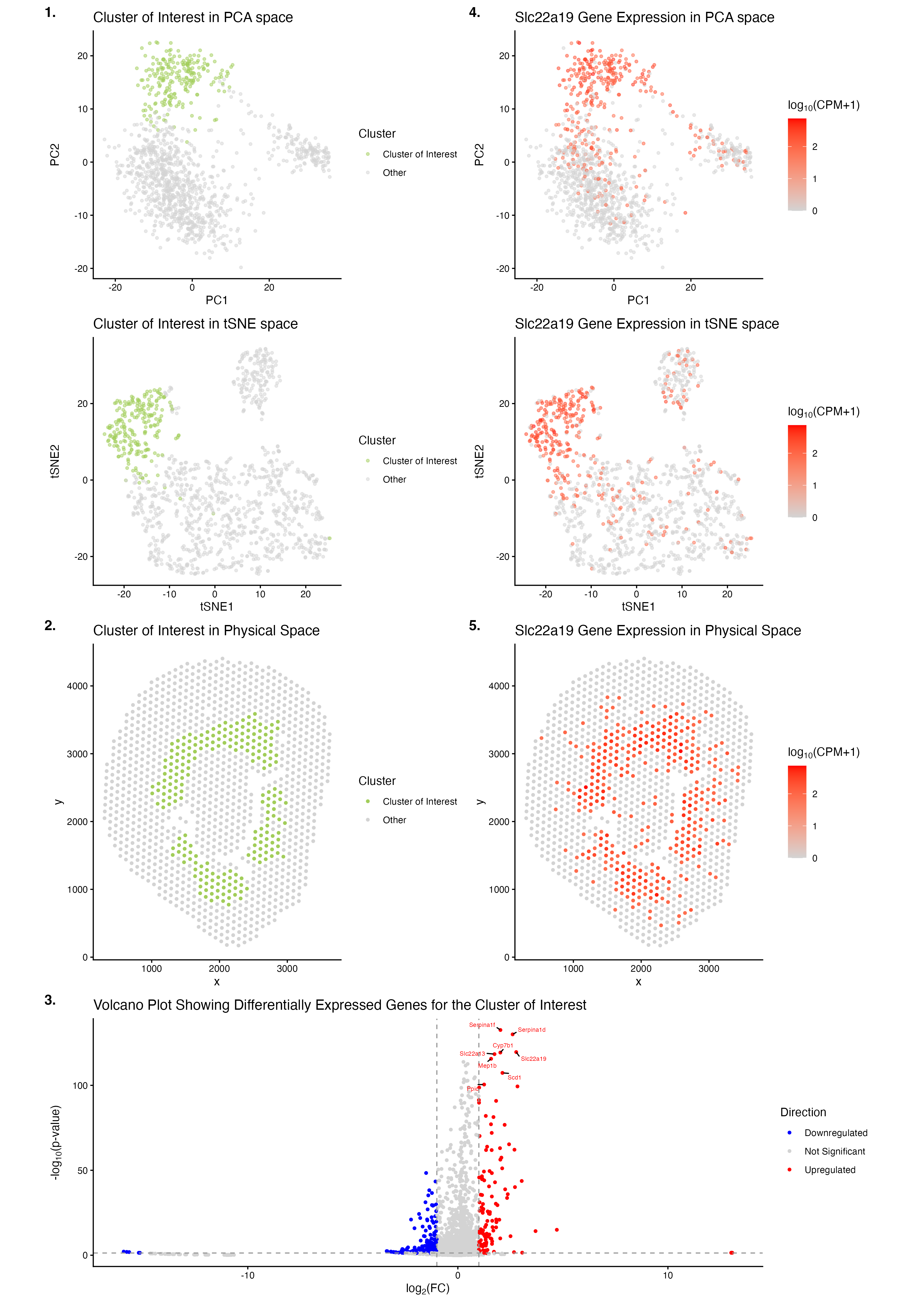
The figure identifies the Cluster of Interest as a coherent, transcriptionally distinct, and spatially localized cluster of cells in the Visium data. K-means clustering was performed using k (centers) = 6, as this optimal value was the k at the elbow of the scree plot depicting total withinness on the y-axis and number of centroids k on the x-axis. Initial examination of the reduced dimensional space of PCA led to the selection of Cluster 6 as the Cluster of Interest, as it had minimal overlap with all of the remaining clusters and was distinctly congregated. In panel 1., the Cluster of Interest (olive green) was found to form a distinct cluster of cells in the linearly reduced dimensional space of PCA and the non-linearly reduced dimensional space of tSNE (light grey). In panel 2., the Cluster of Interest (olive green) was found to be concentrated in a spatially localized ring-like region, co-localized to that formed in the other Xenium dataset, implying the marking of an anatomically organized compartment in the physical space (light grey). In panel 3., the Cluster of Interest shows its differentially expressed genes that are upregulated (red; e.g., Serpina1d, Serpina1f, Slc22a19, Cyp7b1, Slc22a13, Mep1b, Scd1, Ppic), not significantly changed in expression (light grey), or downregulated (blue) compared to gene expressions in all of the remaining clusters. Given that Slc22a19 was found to be a differentially upregulated gene in the Cluster of Interest (pval = 2.567588e-120, log2fc = 2.77762136) through the examination of outputs from the two-sided Wilcoxon rank-sum test performed to depict the volcano plot in panel 3., analogous to how this gene was also differentially upregulated in Cluster 8 of the Xenium dataset (pval = 1e-100, log2fc = 4.74521696), it was selected as a potential marker gene for the Cluster of Interest in the Visium dataset. In panel 4., cells that highly express Slc22a19 (red) were found to form a distinct cluster in the linearly reduced dimensional space of PCA and the non-linearly reduced dimensional space of tSNE (light grey); these clusters also spatially co-localized to those formed by the Cluster of Interest in the PCA and tSNE spaces, respectively, indicating the Slc22a19 gene’s role as a marker gene for the Cluster of Interest. In panel 5., cells that highly express Slc22a19 (red) were found to be concentrated in a spatially localized ring-like region, implying the marking of an anatomically organized compartment in the physical space (light grey). This ring-like region is also spatially co-localized to that formed by the Cluster of Interest in the physical space, as well as that formed in the other Xenium dataset, further validating the Slc22a19 gene’s role as a marker gene for the transcriptionally distinct Cluster of Interest in the Visium dataset and Cluster 8 in the Xenium dataset.
The Cluster of Interest in the Visium dataset is speculated to correspond to proximal tubule epithelial cells, which is the same cell-type identified by Cluster 8 in the Xenium dataset. The Slc22a19 gene (encoding the organic anion transporter OAT5), upregulated in both the Cluster of Interest in the Visium dataset and Cluster 8 of the Xenium dataset, has been characterized to be localized to the apical membrane of the S3 segment in renal proximal tubules, within mouse kidneys[1],[2],[3]. Additionally, the Slc7a12 (encoding asc-type amino acid transporter 2) and Cyp7b1 (encoding oxysterol 7-alpha-hydroxylase) genes, both upregulated in the Cluster of Interest in the Visium dataset and Cluster 8 of the Xenium dataset, have been characterized as female-biased and male-biased marker genes of the S3 segment in renal proximal tubules, respectively[4],[5]. Also, the Serpina1f gene (encoding serpin family A member 1F), upregulated in the Cluster of Interest in the Visium dataset, has been characterized to be localized to proximal tubule epithelial cells in male and female mice[6]. Moreover, the Slc22a13 gene (encoding the organic anion transporter OAT10), upregulated in the Cluster of Interest in the Visium dataset, has been characterized to be highly expressed on the apical membrane of renal proximal tubule cells[7],[8],[9],[10]. Furthermore, the Mep1b gene (encoding the beta subunit of meprin A), upregulated in the Cluster of Interest in the Visium dataset, has been characterized to be localized in the apical membranes of renal proximal tubules[11]. Lastly, the Scd1 gene (encoding stearoyl-CoA desaturase-1), upregulated in the Cluster of Interest in the Visium dataset, has been characterized to be highly expressed in the S3 segment of tubular epithelial cells during acute kidney injury[12]. Overall, the anatomical, ring-like localization of the Cluster of Interest in the mouse kidney, and references from the literature that discuss the roles of several highly upregulated gene markers for the Cluster of Interest, strongly support that the Cluster of Interest in the Visium dataset corresponds to the cell-type identity of proximal tubule epithelial cells (most likely in the S3 segment), which is identical to the cell-type found by Cluster 8 in the Xenium dataset.
You will likely need to change your code from HW3. Write a description of what you changed and why you think you had to change it.
First, I increased the point sizes from 0.5 (in HW3) to 1.0 (in HW4) in panels 1., 2., 4., and 5. This is because, given that Visium is a spot-based spatial transcriptomic profiling technique and Xenium is imaging-based, the former provides multi-cellular spot resolution whereas the latter achieves single-cell resolution, hence allowing each point’s size to be increased for clearer visualization (in HW4) as the Visium dataset contains significantly fewer spatial data points (~1000 spots) to be plotted compared to in the Xenium dataset (~80000 cells). Second, I increased the alpha values of the points from 0.5 (in HW3) to 1.0 (in HW4) in panels 2. and 5. This is because, similar to the previous reason, Visium, being a spot-based spatial transcriptomic profiling technique with fewer spatial data points to plot than the imaging-based Xenium, led to no overlaps when plotting the spatial data points in physical space, removing the need to plot using partially transparent points and allowing each point to be displayed fully opaquely. Third, I decreased the number of PCs used to perform tSNE and then K-means clustering from 10 PCs (in HW3) to 7 PCs (in HW4). This is because the multi-cellular spot resolution in the Visium dataset, compared to the single-cell resolution in the Xenium dataset, can lead to averaging gene expression across cells per spot. In turn, this tends to reduce the amplitude of cell-type-specific differences, leading to fewer dominant PC axes to capture much of the variance, and the scree plot depicting loading on the y-axis and PC index on the x-axis drops sharply then flattens sooner in the Visium dataset, resulting in a smaller optimal PC index, which does not introduce low-variance, noisy PCs, at the elbow of the scree plot compared to the Xenium dataset. Fourth, I decreased the number of centroids from k = 10 (in HW3) to k = 6 (in HW4) and changed the cluster of interest from Cluster 8 (in HW3) to Cluster 6 (in HW4). This is because of the previous reason as well, leading to fewer sharply separable clusters of cells in the Visium dataset than in the Xenium dataset. In turn, this leads to fewer centroids needed to capture much of the total withinness, and the scree plot of total withinness on the y-axis and number of centroids k on the x-axis drops sharply, then flattens sooner in the Visium dataset, yielding a smaller optimal number of centroids at the elbow of the scree plot compared to the Xenium dataset. As a result, the corresponding cluster of interest representing the same cell-type was assigned a different numeric label in the Visium dataset from the Xenium dataset, but their matching identities were validated by the enrichment of similar genetic markers and matching localization patterns in physical space. Fifth, I changed the thresholds for gene name labeling in panel 3. (volcano plot) from abs(log2fc) > 3.5 & neglog10p > 250 (in HW3) to abs(log2fc) > 1 & neglog10p > 100 (in HW4), because the fold-changes in the latter Visium dataset are often compressed and smaller in differential extent due to their lower, multi-cellular spot resolution in comparison to the higher, single-cell resolution in the Xenium dataset, as discussed above. Sixth, to refine my data visualization based on the feedback I received to HW3, I have altered the legend titles in panels 4. and 5. from “Slc22a19 Gene Expression” (in HW3) to “log10(CPM+1)” (in HW4), in order to note the scale used when a transformation has been performed on the gene expression data; additionally, I have altered the cluster of interest’s naming from “cluster_8” (in HW3) to “Cluster of Interest” (in HW4) to remove any confusions that may be caused by pinpointing a specific numeric label, when the numeric labels for all other clusters beyond the cluster of interest are not shown.
[1] https://doi.org/10.14670/HH-25.1385
[2] https://doi.org/10.1152/ajprenal.00012.2004
[3] https://doi.org/10.1124/jpet.105.088583
[4] https://doi.org/10.1073/pnas.2026684118
[5] https://doi.org/10.1016/j.devcel.2019.10.005
[6] https://doi.org/10.1101/2025.11.21.689845
[7] https://www.proteinatlas.org/ENSG00000172940-SLC22A13
[8] https://doi.org/10.1074/jbc.M800737200
[9] https://doi.org/10.1136/annrheumdis-2019-216044
[10] https://doi.org/10.1016/j.dmpk.2021.100443
[11] https://doi.org/10.1074/jbc.M114.559088
[12] https://doi.org/10.1681/ASN.2024znx22t4j
Code
1
2
3
4
5
6
7
8
9
10
11
12
13
14
15
16
17
18
19
20
21
22
23
24
25
26
27
28
29
30
31
32
33
34
35
36
37
38
39
40
41
42
43
44
45
46
47
48
49
50
51
52
53
54
55
56
57
58
59
60
61
62
63
64
65
66
67
68
69
70
71
72
73
74
75
76
77
78
79
80
81
82
83
84
85
86
87
88
89
90
91
92
93
94
95
96
97
98
99
100
101
102
103
104
105
106
107
108
109
110
111
112
113
114
115
116
117
118
119
120
121
122
123
124
125
126
127
128
129
130
131
132
133
134
135
136
137
138
139
140
141
142
143
144
145
146
147
148
149
150
151
152
153
154
155
156
157
158
159
160
161
162
163
164
165
166
167
168
169
170
171
172
173
174
175
176
177
178
179
180
181
182
183
184
185
186
187
188
189
190
191
192
193
194
195
196
197
198
199
200
201
202
203
204
205
206
207
208
209
# Load the necessary libraries
library(ggplot2)
library(ggrepel)
library(patchwork)

# Read in data
data <- read.csv('~/Documents/genomic-data-visualization-2026/data/Visium-IRI-ShamR_matrix.csv.gz')
pos <- data[,c('x', 'y')]
rownames(pos) <- data[,1]
gexp <- data[, 4:ncol(data)]
rownames(gexp) <- data[,1]

# Normalize
totgexp <- rowSums(gexp)
mat <- log10(gexp/totgexp * 1e6 + 1)

# PCA: linear dimensionality reduction
pcs <- prcomp(mat, center=TRUE, scale=FALSE)
plot(pcs$sdev[1:50]) # Scree plot: Will perform tSNE on top 7 PCs as it reaches the elbow of the graph

# tSNE: non-linear dimensionality reduction
set.seed(21726)
tsne <- Rtsne::Rtsne(pcs$x[, 1:7], dims=2, perplexity=30, verbose=TRUE)
emb <- tsne$Y
rownames(emb) <- rownames(mat)
colnames(emb) <- c('tSNE1', 'tSNE2')

# Determining the optimal k value for K-means clustering
totw <- sapply(2:25, function(k) {kmeans(pcs$x[,1:7], centers = k, nstart = 10, iter.max = 500, algorithm = "Lloyd")$tot.withinss})
df_totw <- data.frame(k = 2:25, tot.withinss = totw)
ggplot(df_totw, aes(x = k, y = tot.withinss)) + geom_point() + geom_line() + theme_test() # Scree plot: Optimal k = 6 found for K-means clustering

# K-means clustering
clusters <- as.factor(kmeans(pcs$x[,1:7], centers = 6)$cluster)
df_km <- data.frame(pcs$x, clusters)
ggplot(df_km, aes(x=PC1, y=PC2, col=clusters)) + geom_point(size = 1.0) # PC1 vs PC2: Selected cluster 6 as the one transcriptionally distinct cluster of interest (cells)

# Define labels for cluster of interest (cluster 6) versus other clusters
cluster_label <- ifelse(clusters == 6, "Cluster of Interest", "Other")
clusterofinterest <- clusters == "6"
othercells <- clusters != "6"

# Define colors for cluster of interest (cluster 6) versus other clusters
cluster.cols <- c("Other" = "lightgrey", "Cluster of Interest" = "darkolivegreen3")

# 1. Plot a panel visualizing cluster of interest (cluster 6) in reduced dimensional space (PCA)
df_pca_cluster_6 <- data.frame(
  pcs$x,
  cluster = factor(cluster_label, levels = c("Cluster of Interest", "Other"))
)
p1 <- ggplot(df_pca_cluster_6, aes(x = PC1, y = PC2, color = cluster)) +
  geom_point(size = 1.0, alpha = 0.5) +
  theme_classic() +
  scale_color_manual(values = cluster.cols) +
  labs(title = "Cluster of Interest in PCA space",
       x = "PC1", y = "PC2", color = "Cluster")

# 1. Plot a panel visualizing cluster of interest (cluster 6) in reduced dimensional space (tSNE)
df_tsne_cluster_6 <- data.frame(
  emb1 = emb[, 1],
  emb2 = emb[, 2],
  cluster = factor(cluster_label, levels = c("Cluster of Interest", "Other"))
)
p2 <- ggplot(df_tsne_cluster_6, aes(x = emb1, y = emb2, color = cluster)) +
  geom_point(size = 1.0, alpha = 0.5) +
  theme_classic() +
  scale_color_manual(values = cluster.cols) +
  labs(title = "Cluster of Interest in tSNE space",
       x = "tSNE1", y = "tSNE2", color = "Cluster")

# 2. Plot a panel visualizing cluster of interest (cluster 6) in physical space
df_phys_cluster_6 <- data.frame(
  x = pos[, 1],
  y = pos[, 2],
  cluster = factor(cluster_label, levels = c("Cluster of Interest", "Other"))
)
p3 <- ggplot(df_phys_cluster_6, aes(x = x, y = y, color = cluster)) +
  geom_point(size = 1.0) +
  theme_classic() +
  scale_color_manual(values = cluster.cols) +
  coord_fixed() +
  labs(title = "Cluster of Interest in Physical Space",
       x = "x", y = "y", color = "Cluster")

# Compute Wilcoxon p-values (two-sided for volcano plot)
pv <- sapply(colnames(mat), function(gene) {
  x1 <- mat[clusterofinterest, gene]
  x2 <- mat[othercells, gene]
  wilcox.test(x1, x2, alternative = "two.sided")$p.value
})

# Treat un-testable genes as not significant
pv[is.na(pv)] <- 1
# Avoid p-values of zeros
pv[pv == 0] <- 1e-300

# Compute log2 fold-change
logfc <- sapply(colnames(mat), function(gene) {
  log2((mean(mat[clusterofinterest, gene]) + 1e-6) / (mean(mat[othercells, gene]) + 1e-6))
})

# 3. Plot a panel (volcano plot) visualizing differentially expressed genes for cluster of interest (cluster 6)
de <- data.frame(gene = colnames(mat), pval = pv, neglog10p = -log10(pv), log2fc = logfc)
de$status <- "Not Significant"
de$status[de$pval < 0.05 & de$log2fc > 1]  <- "Upregulated"
de$status[de$pval < 0.05 & de$log2fc < -1] <- "Downregulated"
p4 <- ggplot(de, aes(x = log2fc, y = neglog10p, color = status)) +
  geom_point(size = 1.0) +
  geom_vline(xintercept = c(-1, 1), linetype = "dashed", color = "grey60") +
  geom_hline(yintercept = -log10(0.05), linetype = "dashed", color = "grey60") +
  scale_color_manual(values = c("Downregulated" = "blue",
                                "Not Significant" = "lightgrey",
                                "Upregulated" = "red")) +
  theme_classic() +
  labs(
    title = "Volcano Plot Showing Differentially Expressed Genes for the Cluster of Interest",
    x = expression("log"[2]*"(FC)"),
    y = expression("-log"[10]*"(p-value)"),
    color = "Direction"
  ) +
  geom_text_repel(
    data = subset(de, abs(log2fc) > 1 & neglog10p > 100),
    aes(label = gene),
    size = 2,
    max.overlaps = 20,
    show.legend = FALSE,
    segment.color = "black",
    segment.size = 0.5,
    min.segment.length = 0
  )

# Show top DE genes: selected Slc22a19 as a DE gene from this output (pval = 2.567588e-120, log2fc = 2.77762136, status = Upregulated)
de[order(de$pval), ]

# 4. Plot a panel visualizing the Slc22a19 gene in reduced dimensional space (PCA)
df_pca_Slc22a19 <- data.frame(
  pcs$x,
  gene = mat[, 'Slc22a19']
)
p5 <- ggplot(df_pca_Slc22a19, aes(x = PC1, y = PC2, color = gene)) +
  geom_point(size = 1.0, alpha = 0.5) +
  theme_classic() +
  scale_color_gradient(low='lightgrey', high='red') +
  labs(
    title = "Slc22a19 Gene Expression in PCA space",
    x = "PC1", y = "PC2", color = expression("log"[10]*"(CPM+1)")
  )

# 4. Plot a panel visualizing the Slc22a19 gene in reduced dimensional space (tSNE)
df_tsne_Slc22a19 <- data.frame(
  emb1 = emb[, 1],
  emb2 = emb[, 2],
  gene = mat[, 'Slc22a19']
)
p6 <- ggplot(df_tsne_Slc22a19, aes(x = emb1, y = emb2, color = gene)) +
  geom_point(size = 1.0, alpha = 0.5) +
  theme_classic() +
  scale_color_gradient(low='lightgrey', high='red') +
  labs(
    title = "Slc22a19 Gene Expression in tSNE space",
    x = "tSNE1", y = "tSNE2", color = expression("log"[10]*"(CPM+1)")
  )

# 5. Plot a panel visualizing the Slc22a19 gene in physical space
df_phys_Slc22a19 <- data.frame(
  x = pos[, 1],
  y = pos[, 2],
  gene = mat[, 'Slc22a19']
)

p7 <- ggplot(df_phys_Slc22a19, aes(x = x, y = y, color = gene)) +
  geom_point(size = 1.0) +
  theme_classic() +
  coord_fixed() +
  scale_color_gradient(low='lightgrey', high='red') +
  labs(
    title = "Slc22a19 Gene Expression in Physical Space",
    x = "x", y = "y", color = expression("log"[10]*"(CPM+1)")
  )

# Plot all panels in one plot using patchwork
p1_tag <- p1 + labs(tag = "1.")
p3_tag <- p3 + labs(tag = "2.")
p4_tag <- p4 + labs(tag = "3.")
p5_tag <- p5 + labs(tag = "4.")
p7_tag <- p7 + labs(tag = "5.")
tag_theme <- theme(
  plot.tag.position = c(0, 1),
  plot.tag = element_text(face = "bold")
)
p1_tag <- p1_tag + tag_theme
p3_tag <- p3_tag + tag_theme
p4_tag <- p4_tag + tag_theme
p5_tag <- p5_tag + tag_theme
p7_tag <- p7_tag + tag_theme
plot.layout <- "
AB
CD
EF
GG
"
p_all <-
  p1_tag + p5_tag +
  p2 + p6 +
  p3_tag + p7_tag +
  p4_tag +
  plot_layout(design = plot.layout)
p_all
ggsave("hw4_yhodo1.png", p_all, width = 12, height = 17, dpi = 300)