HW 4

Hi! I'm Anna! I'm a senior BME, and I'm excited to learn more about data visualizations.

Write a description to convince me you found the same cell-type.

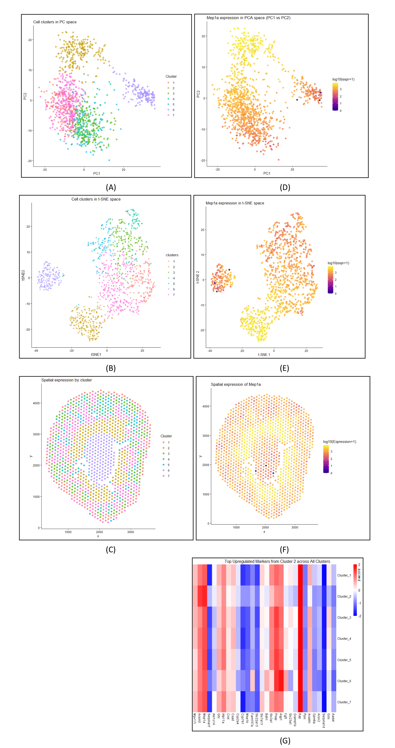
Cluster 2 most likely represents proximal tubule S3 epithelial cells. This is supported by its inner stripe/outer medulla location highlighted in yellow in Panel C/F and Mep1a’s high expression in the same area in PCA and tSNE plots (Panels A/D and Panels B/E), matching a brush-border proximal tubule pattern. Additionally, the heatmap (Panel G) shows Mep1a rising alongside other transport/energy genes like Aqp1 and Acsm3, indicating a coordinated proximal tubule program. This aligns with a study by Herzog et al., which shows that meprin A (Mep1a) is a brush-border enzyme in proximal tubules and changes with acute kidney injury, reinforcing its S3 proximal tubule identity. https://pubmed.ncbi.nlm.nih.gov/17377510/

Write a description of what you changed and why you think you had to change it.

Using the Visium dataset, I normalized and log-transformed the data and performed PCA, in which the scree plot showed 5 points before the “elbow” of the plot. Previously, in the Xenium dataset, the scree plot included 9 points before reaching the “elbow” of the plot, but 9 pcs on the Visium dataset would have been redundant. Additionally, I performed t-SNE on the top 10 PCs because I wanted to better visualize the clusters and any local patterns, which I had not done previously.

I previously performed k-means clustering with k=8 on the Xenium dataset. With the Visium dataset, I performed k-means clustering with k=5. This is because I found the optimal K based on total-withinness to be only 5 for this dataset. One possible reason there is a lower optimal number of transcriptionally distinct cell clusters in the spot-based dataset compared to the single-cell resolution dataset is that in Visium, each spot mixes signals from multiple cells, potentially showing smoother patterns. Therefore, the Visium data could form fewer, broader groups, whereas finer clustering is needed for single-cell data.

Additionally, I changed the potential marker for Cluster 2 from Slc7a13 to Mep1a because, in the Xenium dataset, Slc7a13 often bled outside its cluster and wasn’t exclusive, making it less reliable as a defining marker. When observing Mep1a, it showed a stronger, more localized gene expression in Cluster 2 with the high z-score on the heatmap and aligned with the cluster’s PCA/t-SNE plots, indicating greater specificity.

Code

# Read in data
data <- read.csv("Visium-IRI-ShamR_matrix.csv.gz") 
data[1:5, 1:5]
pos <- data[, c('x', 'y')]
rownames(pos) <- data[,1]
gexp <- data[, 4:ncol(data)]
rownames(gexp) <- data[,1]

# Normalize and log transform data 
totgexp <- rowSums(gexp)
head(totgexp)
head(sort(totgexp, decreasing=TRUE))
mat <- log10(gexp / totgexp * 1e6 + 1 ) 
dim(mat) # 1224 19465

# PCA
## no scaling 
pcs <- prcomp(mat, center=TRUE, scale=FALSE) 
names(pcs)
head(pcs$sdev)
length(pcs$sdev)
plot(pcs$sdev[1:50]) # scree plot reveals 5 points before the elbow 
pc_scores <- pcs$x[, 1:4, drop=FALSE]
colnames(pc_scores) <- paste0("PC", 1:4)


# conduct tSNE
library(Rtsne)
pcs_use <- pcs$x[, 1:10, drop = FALSE]
tsne_out <- Rtsne(pcs_use, perplexity = 30, theta = 0.5, verbose = TRUE, check_duplicates = FALSE)


# determine k-centroids through scree plot
wcss <- wss <- sapply(2:12, function(k) {
kmeans(pcs_use, centers = k, nstart = 50, iter.max = 100)$tot.withinss
})
k_centroids <- 1:50 

scree_df <- data.frame(
  k = k_centroids,
  wcss = wcss # makes no sense
)

scree_plot <- ggplot(scree_df, aes(x = k, y = wcss)) +
  geom_line() +
  geom_point(size = 2) +
  labs(
    title = "Scree plot for choosing k-centroids",
    x = "Number of clusters",
    y = "Total within-cluster Sum of Squares"
  ) +
  theme_classic() +
  theme(plot.title = element_text(size = 11))


# choose top 5 PCs 
pcs_use <- pcs$x[, 1:5, drop=FALSE]

# run k-means 
set.seed(123)
km <- kmeans(pcs_use, centers = 7, nstart = 100, iter.max = 300)
clusters <- factor(km$cluster)

df <- data.frame(
  pcs$x[, 1:2, drop = FALSE], 
  clusters
)

# compute the centroid
centroid_pcs <- aggregate(cbind(PC1, PC2) ~ clusters, data = df, FUN = median)

# panel B
cell_cluster_pc <- ggplot(df, aes(PC1, PC2, color = clusters)) +
geom_point(alpha = 0.6, size = 2) +
labs(title = "All Clusters in PCA", x = "PC1", y = "PC2", color = "Cluster") +
theme_classic()

# panel c
# tsne coordinates
embedding_coords <- tsne_out$Y
colnames(embedding_coords) <- c("tSNE1", "tSNE2")  

df <- data.frame(
    tSNE1 = embedding_coords[,1],
    tSNE2 = embedding_coords[,2],
    clusters = factor(clusters)
)

# compute centroids for tsne
centroid_tsne <- aggregate(cbind(tSNE1, tSNE2) ~ clusters, data = df, FUN = median)

p_tsne <- ggplot(df, aes(tSNE1, tSNE2, color = clusters)) +
geom_point(alpha = 0.5) +
labs(title = "All Clusters in t-SNE space") +
theme_classic() +
theme(plot.title = element_text(hjust = 0.5))

# panel d

# Ensure clusters is a factor and aligned with pos
clusters_f <- factor(clusters[rownames(pos)])

# Data frame for plotting
df_sp <- data.frame(x = pos$x, y = pos$y, cluster = clusters_f)

# Spatial plot colored by cluster
ggplot(df_sp, aes(x, y, color = cluster)) +
  geom_point(size = 2, alpha = 0.8) +
  coord_equal() +
  labs(title = "Spatial expression by cluster", x = "x", y = "y", color = "Cluster") +
  theme_classic()

# Determined through the spatial expression that the cluster of interest is cluster 2 
# as it has a very similiar spatial expression as the cluster of interest in HW3



# set up df for differential expression 
library(matrixStats)
# trying to characterize cluster 2:

# Used AI: Prompt: help me identify genes upregulated in cluster 2 
# vs all other clusters using a Wilcoxon rank-sum test on log-normalized data

# identify upregulated genes in cluster 2  vs other clusters
# Align to common cells to avoid mismatches
common_cells <- intersect(rownames(mat), names(clusters))
mat_use <- mat[common_cells, , drop = FALSE]
clusters_use <- clusters[common_cells]
genes <- colnames(mat_use)

# Define cluster 2 vs rest
cl_cells <- names(clusters_use)[clusters_use == 2]
ot_cells <- names(clusters_use)[clusters_use != 2]
# Extract matrices
mat_in  <- mat_use[cl_cells, genes, drop = FALSE]
mat_out <- mat_use[ot_cells, genes, drop = FALSE]
# Wilcoxon rank-sum p-values (upregulated in cluster 2)
wilcox_p <- sapply(genes, function(g) {
wilcox.test(mat_in[, g], mat_out[, g], alternative = "greater")$p.value
})
wilcox_fdr <- p.adjust(wilcox_p, method = "BH")
# expression threshold
expr_threshold = log10(2)
# Effect sizes
mean_diff <- colMeans(mat_in) - colMeans(mat_out)           # magnitude on log scale
pct_in    <- colMeans(mat_in  > expr_threshold)             # detection in cluster 7
pct_out   <- colMeans(mat_out > expr_threshold)             # detection outside
pct_diff  <- pct_in - pct_out
auroc     <- sapply(genes, function(g) auroc_gene(mat_in[, g], mat_out[, g]))  # separation
# Assemble results table
de_2 <- data.frame(
gene = genes,
wilcox_p = wilcox_p,
wilcox_fdr = wilcox_fdr,
mean_diff = mean_diff,
pct_in = pct_in,
pct_out = pct_out,
pct_diff = pct_diff,
stringsAsFactors = FALSE
)

# Used AI to add in auroc
# Prompt: How could I compute AUROC per gene?
# add in auroc
auroc_gene <- function(x_in, x_out) {
n_in <- length(x_in); n_out <- length(x_out)
r <- rank(c(x_in, x_out)) # average ranks for ties
U <- sum(r[1:n_in]) - n_in * (n_in + 1) / 2
U / (n_in * n_out) # AUC in [0,1]
}

de_2$auroc <- sapply(genes, function(g) auroc_gene(mat_in[, g], mat_out[, g]))


# Keep upregulated, significant genes and rank by strength (AUROC, then pct_diff, then mean_diff)
markers_2 <- subset(de_2, wilcox_fdr < 0.05 & mean_diff > 0)
markers_2 <- markers_2[order(-markers_2$auroc, -markers_2$pct_diff, -markers_2$mean_diff), ]
head(markers_2, 20)

# plot heatmap of cluster-averaged expression for top markers
# select top N upregulated markers for cluster 2
topN <- 30
top_genes <- head(markers_2$gene, topN)
top_genes <- top_genes[top_genes %in% colnames(mat)]  # ensure present

# compute average expression per cluster for these genes
cl_levels <- sort(unique(clusters))

avg_by_cluster <- sapply(cl_levels, function(c) {
  cells_c <- names(clusters)[clusters == c]
  colMeans(mat[cells_c, top_genes, drop = FALSE])
})

# transform so that clusters are rows and genes are columns
avg_by_cluster <- t(avg_by_cluster)

colnames(avg_by_cluster) <- top_genes
rownames(avg_by_cluster) <- paste0("Cluster_", cl_levels)

# z-score genes across clusters 
# purpose: make genes comparable versus using raw values for gene expression
z <- t(scale(t(avg_by_cluster)))

# Define color scale: blue (neg) → white (0) → red (pos)
# used AI to revise the look of the heat map
# prompt: could you revise this code so that the cluster labels are on the 
# left side of the y-axis and that the gene labels are read from left to right. 
# additionally, add a label for the legend "z-score" and set white = 0 with positive 
# z score at red and negative at blue. additionally, remove clustering tree
library(pheatmap)
heatmap_plot <- pheatmap(
  z,
  cluster_rows = FALSE,      # remove dendrogram (tree) for clusters
  cluster_cols = FALSE,      # remove dendrogram for genes
  color = colorRampPalette(c("blue", "white", "red"))(100),
  breaks = seq(-2, 2, length.out = 101),   # ensures white centered at 0
  main = "",
  fontsize_row = 9,
  fontsize_col = 9,
  border_color = NA
)
# add legend title "z-score"
library(grid)
grid::grid.text("z-score", x = unit(0.97, "npc"), y = unit(0.9, "npc"), rot = 90, gp = gpar(cex = 0.9))

# add custom title
grid.text(
  "Top Upregulated Markers from Cluster 2 across All Clusters",
  x = 0.5,
  y = 0.98,
  gp = gpar(fontsize = 12, fontface = "plain")
)

ggsave("heatmap_plot.png", heatmap_plot, width = 6, height = 5, dpi = 300)

# Double check that Mep1a is differentially upregulated 
# Define cluster 2 vs rest
cl2 <- names(clusters)[clusters == 2]
other <- names(clusters)[clusters != 2]

# Extract expression for Mep1a (log10 CPM+1)
x1 <- mat[cl2, "Mep1a"]
x2 <- mat[other, "Mep1a"]

# Wilcoxon rank-sum test (upregulated in cluster 2)
wilcox_p <- wilcox.test(x1, x2, alternative = "greater")$p.value
wilcox_fdr <- p.adjust(wilcox_p, method = "BH")

# Effect sizes
logFC <- mean(x1) - mean(x2)
thr <- log10(2)
pct_in  <- mean(x1 > thr)
pct_out <- mean(x2 > thr)

# Print a brief summary
cat("Mep1a: p =", wilcox_p, "FDR =", wilcox_fdr,
    "logFC =", round(logFC, 3),
    "pct_in =", round(pct_in, 2),
    "pct_out =", round(pct_out, 2), "\n")


# visualize Mep1a in reduced dimensional space (PCA)
Mep1a_df <- data.frame(PC1 = pcs$x[,1], PC2 = pcs$x[,2], Mep1a = mat[, "Mep1a"])

# panel E
# Mep1a
rng <- range(Mep1a_df$Mep1a, na.rm = TRUE)
ggplot(Mep1a_df, aes(PC1, PC2, color = Mep1a)) +
geom_point(size = 2, alpha = 0.8) +
labs(title = "Mep1a expression in PCA space (PC1 vs PC2)", x = "PC1", y = "PC2") +
scale_color_viridis_c(option = "C", limits = rng, name = "log10(expr+1)") +
theme_classic()

# panel f
ggplot(Mep1a_spatial_df, aes(x, y, color = Mep1a)) +
geom_point(size = 2, alpha = 0.8) +
scale_color_viridis_c(option = "C", limits = rng, name = "log10(Expression+1)") +
labs(title = "Spatial expression of Mep1a", x = "x", y = "y") +
coord_equal() + theme_classic()

# panel g
colnames(embedding_coords) <- c("tSNE1", "tSNE2")
df_tsne <- data.frame(tSNE1 = embedding_coords[,1], tSNE2 = embedding_coords[,2], Mep1a = mat[, "Mep1a"])

ggplot(df_tsne, aes(tSNE1, tSNE2, color = Mep1a)) +
  geom_point(size = 2, alpha = 0.8) +
  scale_color_viridis_c(option = "C", name = "log10(expr+1)") +
  labs(title = "Mep1a expression in t-SNE space", x = "t-SNE 1", y = "t-SNE 2") +
  theme_classic()

17 Feb 2026

« HW4: Multi-Panel Data Visualization of a Transcriptionally Distinct Proximal Tubule Epithelial Cell Cluster in the Visium Dataset Adapting Cell Type Characterization from Visium Dataset to Xenium Dataset »