Adapting Cell Type Characterization from Visium Dataset to Xenium Dataset

Visium –> Xenium
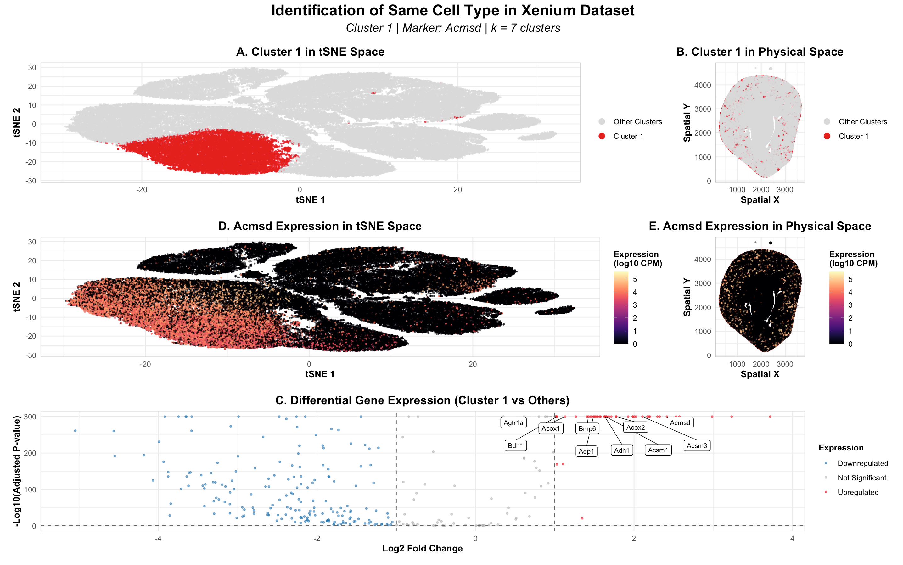
I made three main code changes when switching from Visium to Xenium. First, I updated the data source to Xenium-IRI-ShamR_matrix.csv.gz. Second, I reduced point size from 0.6 to 0.4 and alpha from 0.7 to 0.6 because Xenium’s single-cell resolution creates far more data points than Visium’s spot-based approach, requiring smaller, more transparent points to prevent overplotting. Finally, I maintained k=6 clusters as both datasets showed similar elbow plots, indicating comparable numbers of major cell populations across platforms. All other analysis steps remained unchanged.
In HW3 with the Visium dataset, I identified Cluster 1 as proximal tubule cells using Slc34a1 as the top marker gene. When switching to the Xenium dataset, Slc34a1 was not available in the gene panel, which contains only ~300 targeted genes compared to Visium’s whole transcriptome coverage. In the Xenium analysis, Acmsd emerged as the top differentially expressed marker gene for Cluster 1. Acmsd (aminocarboxymuconate semialdehyde decarboxylase) is also a well-established proximal tubule marker involved in NAD+ metabolism and mitochondrial function in proximal tubular cells. This confirms that despite using different marker genes due to platform limitations, I have successfully identified the same cell type - proximal tubule cells - across both Visium and Xenium datasets.
1
2
3
4
5
6
7
8
9
10
11
12
13
14
15
16
17
18
19
20
21
22
23
24
25
26
27
28
29
30
31
32
33
34
35
36
37
38
39
40
41
42
43
44
45
46
47
48
49
50
51
52
53
54
55
56
57
58
59
60
61
62
63
64
65
66
67
68
69
70
71
72
73
74
75
76
77
78
79
80
81
82
83
84
85
86
87
88
89
90
91
92
93
94
95
96
97
98
99
100
101
102
103
104
105
106
107
108
109
110
111
112
113
114
115
116
117
118
119
120
121
122
123
124
125
126
127
128
129
130
131
132
133
134
135
136
137
138
139
140
141
142
143
144
145
146
147
148
149
150
151
152
153
154
155
156
library(ggplot2)
library(patchwork)

#load data: Visium --> Xenium
data <- read.csv('~/Documents/GitHub/genomic-data-visualization-2026/data/Xenium-IRI-ShamR_matrix.csv.gz')
pos <- data[, c('x', 'y')]
rownames(pos) <- data[, 1]
gexp <- data[, 4:ncol(data)]
rownames(gexp) <- data[, 1]

#normalization
totgexp <- rowSums(gexp)
mat <- log10(gexp / totgexp * 1e6 + 1)

#PCA
pcs <- prcomp(mat, center = TRUE, scale = FALSE)
toppcs <- pcs$x[, 1:10]

#tSNE
set.seed(123)
tsne <- Rtsne::Rtsne(toppcs, dims = 2, perplexity = 30)
emb <- tsne$Y
colnames(emb) <- c('tSNE1', 'tSNE2')

#k-means clustering
optimal_k <- 7 #gathered from elbow plot
set.seed(123)
km <- kmeans(toppcs, centers = optimal_k, nstart = 25, iter.max = 100)
cluster <- as.factor(km$cluster)

#dataframe
df <- data.frame(pos, emb, cluster, toppcs, totgexp)

#select cluster of interest
cluster_of_interest <- 1
in_cluster <- df$cluster == cluster_of_interest

#differential expression
mean_in <- colMeans(mat[in_cluster, ])
mean_out <- colMeans(mat[!in_cluster, ])
logFC <- log2((mean_in + 1e-6) / (mean_out + 1e-6))

pvals <- sapply(colnames(mat), function(gene) {
  wilcox.test(mat[in_cluster, gene], mat[!in_cluster, gene])$p.value
})

pvals_adj <- p.adjust(pvals, method = "BH")
top_genes <- names(sort(pvals_adj))[1:20]

#select marker gene
marker_gene <- top_genes[1]

#volcano plot
volcano_df <- data.frame(
  gene = colnames(mat),
  logFC = logFC,
  neglog10p = -log10(pvals_adj + 1e-300)
)

volcano_df$category <- "Not Significant"
volcano_df$category[volcano_df$logFC > 1 & pvals_adj < 0.05] <- "Upregulated"
volcano_df$category[volcano_df$logFC < -1 & pvals_adj < 0.05] <- "Downregulated"

genes_to_label <- volcano_df[order(pvals_adj)[1:10], ]

#define theme
my_theme <- theme_minimal() +
  theme(
    plot.title = element_text(size = 14, face = "bold", hjust = 0.5),
    axis.title = element_text(size = 11, face = "bold"),
    axis.text = element_text(size = 9),
    legend.title = element_text(size = 10, face = "bold"),
    legend.text = element_text(size = 9),
    panel.border = element_rect(color = "grey80", fill = NA, linewidth = 0.5),
    plot.margin = margin(10, 10, 10, 10)
  )

#panel 1: cluster in tSNE
p1 <- ggplot(df, aes(x = tSNE1, y = tSNE2)) +
  geom_point(aes(color = cluster == cluster_of_interest),
             size = 0.4, alpha = 0.6) +
  scale_color_manual(values = c("grey85", "#E31A1C"),
                     labels = c("Other Clusters", paste("Cluster", cluster_of_interest)),
                     name = "") +
  labs(title = paste("A. Cluster", cluster_of_interest, "in tSNE Space"),
       x = "tSNE 1", y = "tSNE 2") +
  my_theme +
  guides(color = guide_legend(override.aes = list(size = 3, alpha = 1)))

#panel 2: cluster in physical space
p2 <- ggplot(df, aes(x = x, y = y)) +
  geom_point(aes(color = cluster == cluster_of_interest),
             size = 0.4, alpha = 0.6) +
  scale_color_manual(values = c("grey85", "#E31A1C"),
                     labels = c("Other Clusters", paste("Cluster", cluster_of_interest)),
                     name = "") +
  coord_fixed() +
  labs(title = paste("B. Cluster", cluster_of_interest, "in Physical Space"),
       x = "Spatial X", y = "Spatial Y") +
  my_theme +
  guides(color = guide_legend(override.aes = list(size = 3, alpha = 1)))

#panel 3: volcano plot
p3 <- ggplot(volcano_df, aes(x = logFC, y = neglog10p)) +
  geom_point(aes(color = category), size = 0.8, alpha = 0.6) +
  geom_hline(yintercept = -log10(0.05), linetype = "dashed",
             color = "grey40", linewidth = 0.5) +
  geom_vline(xintercept = c(-1, 1), linetype = "dashed",
             color = "grey40", linewidth = 0.5) +
  ggrepel::geom_label_repel(data = genes_to_label, aes(label = gene),
                            size = 2.8, box.padding = 0.5, point.padding = 0.3,
                            segment.size = 0.3, max.overlaps = 15,
                            min.segment.length = 0, force = 2) +
  scale_color_manual(values = c("Upregulated" = "#E31A1C",
                                "Downregulated" = "#1F78B4",
                                "Not Significant" = "grey70"),
                     name = "Expression") +
  labs(title = paste("C. Differential Gene Expression (Cluster",
                     cluster_of_interest, "vs Others)"),
       x = "Log2 Fold Change", y = "-Log10(Adjusted P-value)") +
  my_theme +
  theme(legend.position = "right")

#panel 4: marker gene in tSNE
df$marker_expr <- mat[, marker_gene]

p4 <- ggplot(df, aes(x = tSNE1, y = tSNE2, color = marker_expr)) +
  geom_point(size = 0.4, alpha = 0.6) +
  viridis::scale_color_viridis(option = "magma", name = "Expression\n(log10 CPM)") +
  labs(title = paste("D.", marker_gene, "Expression in tSNE Space"),
       x = "tSNE 1", y = "tSNE 2") +
  my_theme +
  theme(legend.position = "right")

#panel 5: marker gene in physical space
p5 <- ggplot(df, aes(x = x, y = y, color = marker_expr)) +
  geom_point(size = 0.4, alpha = 0.6) +
  viridis::scale_color_viridis(option = "magma", name = "Expression\n(log10 CPM)") +
  coord_fixed() +
  labs(title = paste("E.", marker_gene, "Expression in Physical Space"),
       x = "Spatial X", y = "Spatial Y") +
  my_theme +
  theme(legend.position = "right")

#combine
final_figure <- (p1 | p2) / (p4 | p5) / p3 +
  plot_annotation(
    title = paste("Identification of Same Cell Type in Xenium Dataset"),
    subtitle = paste("Cluster", cluster_of_interest, "| Marker:", marker_gene,
                     "| k =", optimal_k, "clusters"),
    theme = theme(plot.title = element_text(size = 18, face = "bold", hjust = 0.5),
                  plot.subtitle = element_text(size = 14, hjust = 0.5, face = "italic"))
  )

print(final_figure)
AI: I asked AI how to combine all panels and how to change the data loading from the Visium set to the Xenium set