title

Description
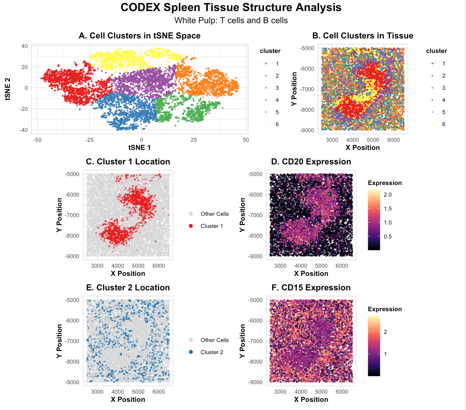
In this analysis, I used CODEX spatial proteomics data from spleen tissue to identify what tissue structure was present. After filtering out low-quality cells by area, I performed tSNE dimensionality reduction and k-means clustering with k=6 to group similar cells together. I then used differential expression analysis to find which proteins were most highly expressed in each cluster. My visualization shows all the cell clusters in tSNE space (panel A) and where they’re located in the actual tissue (panel B), plus the locations and marker expression for two main cell types. Based on the protein markers and how the cells are organized spatially, I identified this tissue as white pulp, the immune region of the spleen.
Cluster 1 has high CD8 expression, which marks these cells as cytotoxic T cells. According to the Human Protein Atlas, CD8 is the standard marker used to identify T cells. These cells are scattered throughout the tissue, which matches the typical pattern of T cell zones in white pulp where T cells move around looking for foreign antigens. Cluster 2 shows high CD20 expression, the main marker for B cells. Unlike the scattered T cells, the B cells are grouped together in concentrated regions, forming organized structures called follicles that normally surround the T cell areas in white pulp.
The fact that I found both CD8+ T cells and CD20+ B cells located together with these specific spatial patterns confirms this is white pulp. White pulp is where the spleen’s immune responses happen, with T cells and B cells working together. I also didn’t find markers for other spleen structures like red pulp (which would show CD68+ macrophages), blood vessels (which would show CD31 and smooth muscle markers), or the structural capsule (which would show collagen at the edges). The CODEX imaging method was key here because it let me see multiple protein markers at once while keeping track of where each cell was located in the tissue.
Sources:
CD8 expression: https://www.proteinatlas.org/ENSG00000153563-CD8A/blood CD20 expression: https://www.proteinatlas.org/ENSG00000112796-MS4A1/blood Spleen anatomy: Mebius RE, Kraal G. Structure and function of the spleen. Nature Reviews Immunology. 2005;5(8):606-616. CODEX imaging: Goltsev Y, et al. Deep Profiling of Mouse Splenic Architecture with CODEX Multiplexed Imaging. Cell. 2018;174(4):968-981.
Code
1
2
3
4
5
6
7
8
9
10
11
12
13
14
15
16
17
18
19
20
21
22
23
24
25
26
27
28
29
30
31
32
33
34
35
36
37
38
39
40
41
42
43
44
45
46
47
48
49
50
51
52
53
54
55
56
57
58
59
60
61
62
63
64
65
66
67
68
69
70
71
72
73
74
75
76
77
78
79
80
81
82
83
84
85
86
87
88
89
90
91
92
93
94
95
96
97
98
99
100
101
102
103
104
105
106
107
108
109
110
111
112
113
114
115
116
117
118
119
120
121
122
123
124
125
126
127
128
129
130
131
132
133
134
135
136
137
138
139
140
141
142
143
144
145
146
147
148
149
150
151
152
153
154
155
156
157
158
159
160
161
162
163
164
165
166
167
168
169
170
data <- read.csv('~/Documents/GitHub/genomic-data-visualization-2026/data/codex_spleen2.csv.gz')

library(ggplot2)
library(patchwork)
dim(data)
pos <- data[, 2:3]
rownames(pos) <- data[, 1]
area <- data[, 4]
names(area) <- data[, 1]
pexp <- data[, 5:ncol(data)]
rownames(pexp) <- data[, 1]

#quality control - get rid of cells that are too small or too large
valid_cells <- area > 50 & area < 500
pos <- pos[valid_cells, ]
area <- area[valid_cells]
pexp <- pexp[valid_cells, ]

#normalize
mat <- log10(pexp / area + 1)

#dimensionality reduction with tSNE
set.seed(123)
emb <- Rtsne::Rtsne(mat)
embedding <- emb$Y
colnames(embedding) <- c('tSNE1', 'tSNE2')
rownames(embedding) <- rownames(mat)

#k-means clustering on tSNE coordinates
set.seed(123)
optimal_k <- 6
km <- kmeans(embedding, centers = optimal_k, nstart = 25, iter.max = 100)
cluster <- as.factor(km$cluster)

#data frame
df <- data.frame(pos, tSNE1 = embedding[,1], tSNE2 = embedding[,2], cluster, area)
cluster1 <- 1
cluster2 <- 2

#find top markers for a cluster
find_markers <- function(cluster_num) {
  in_cluster <- cluster == cluster_num
  mean_in <- colMeans(mat[in_cluster, ])
  mean_out <- colMeans(mat[!in_cluster, ])
  logFC <- log2((mean_in + 1e-6) / (mean_out + 1e-6))

  pvals <- sapply(colnames(mat), function(protein) {
    wilcox.test(mat[in_cluster, protein], mat[!in_cluster, protein])$p.value
  })

  pvals_adj <- p.adjust(pvals, method = "BH")

  results <- data.frame(
    protein = colnames(mat),
    logFC = logFC,
    pval_adj = pvals_adj
  )

  results[order(results$pval_adj), ]
}

#top markers for both clusters
markers_c1 <- find_markers(cluster1)
markers_c2 <- find_markers(cluster2)

#select top marker proteins
marker1 <- markers_c1$protein[1]
marker2 <- markers_c2$protein[1]

#define theme
my_theme <- theme_minimal() +
  theme(
    plot.title = element_text(size = 12, face = "bold", hjust = 0.5),
    axis.title = element_text(size = 10, face = "bold"),
    axis.text = element_text(size = 8),
    legend.title = element_text(size = 9, face = "bold"),
    legend.text = element_text(size = 8),
    panel.border = element_rect(color = "grey80", fill = NA, linewidth = 0.5),
    plot.margin = margin(5, 5, 5, 5)
  )

#panel 1: all clusters in tSNE space
p1 <- ggplot(df, aes(x = tSNE1, y = tSNE2, col = cluster)) +
  geom_point(size = 0.5, alpha = 0.7) +
  scale_color_brewer(palette = "Set1") +
  labs(title = "A. Cell Clusters in tSNE Space",
       x = "tSNE 1", y = "tSNE 2") +
  my_theme


#panel 2: all clusters in physical space
p2 <- ggplot(df, aes(x = x, y = y, col = cluster)) +
  geom_point(size = 0.5, alpha = 0.7) +
  scale_color_brewer(palette = "Set1") +
  coord_fixed() +
  labs(title = "B. Cell Clusters in Tissue",
       x = "X Position", y = "Y Position") +
  my_theme

#panel 3: cluster 1 location
p3 <- ggplot(df, aes(x = x, y = y)) +
  geom_point(aes(color = cluster == cluster1), size = 0.5, alpha = 0.7) +
  scale_color_manual(values = c("grey85", "#E31A1C"),
                     labels = c("Other Cells", paste("Cluster", cluster1)),
                     name = "") +
  coord_fixed() +
  labs(title = paste("C. Cluster", cluster1, "Location"),
       x = "X Position", y = "Y Position") +
  my_theme +
  guides(color = guide_legend(override.aes = list(size = 2, alpha = 1)))

#panel 4: marker 1 expression
df$marker1_expr <- mat[, marker1]
p4 <- ggplot(df, aes(x = x, y = y, color = marker1_expr)) +
  geom_point(size = 0.5, alpha = 0.7) +
  viridis::scale_color_viridis(option = "magma", name = "Expression") +
  coord_fixed() +
  labs(title = paste("D.", marker1, "Expression"),
       x = "X Position", y = "Y Position") +
  my_theme

#panel 5: cluster 2 location
p5 <- ggplot(df, aes(x = x, y = y)) +
  geom_point(aes(color = cluster == cluster2), size = 0.5, alpha = 0.7) +
  scale_color_manual(values = c("grey85", "#1F78B4"),
                     labels = c("Other Cells", paste("Cluster", cluster2)),
                     name = "") +
  coord_fixed() +
  labs(title = paste("E. Cluster", cluster2, "Location"),
       x = "X Position", y = "Y Position") +
  my_theme +
  guides(color = guide_legend(override.aes = list(size = 2, alpha = 1)))

#panel 6: marker 2 expression
df$marker2_expr <- mat[, marker2]
p6 <- ggplot(df, aes(x = x, y = y, color = marker2_expr)) +
  geom_point(size = 0.5, alpha = 0.7) +
  viridis::scale_color_viridis(option = "magma", name = "Expression") +
  coord_fixed() +
  labs(title = paste("F.", marker2, "Expression"),
       x = "X Position", y = "Y Position") +
  my_theme

#combine all panels
final_figure <- (p1 | p2) / (p3 | p4) / (p5 | p6) +
  plot_annotation(
    title = "CODEX Spleen Tissue Structure Analysis",
    subtitle = "White Pulp: T cells and B cells",
    theme = theme(plot.title = element_text(size = 16, face = "bold", hjust = 0.5),
                  plot.subtitle = element_text(size = 12, hjust = 0.5))
  )

print(final_figure)

#save figure
ggsave("hw5_tissue_analysis.png", plot = final_figure,
       width = 12, height = 14, dpi = 300, bg = "white")

#print top markers for reference
print("Top 5 markers for Cluster 1:")
print(head(markers_c1, 5))

print("Top 5 markers for Cluster 2:")
print(head(markers_c2, 5))


## AI Prompts
# given this codex spleen dataset, how do i choose the clusters to emphasize after running tSNE? what plots should i include in analysis?