Identification of CODEX data as White Pulp

Perform a full analysis (quality control, dimensionality reduction, kmeans clustering, differential expression analysis) on your data. Your goal is to figure out what tissue structure is represented in the CODEX data. Options include: (1) Artery/Vein, (2) White pulp, (3) Red pulp, (4) Capsule/Trabecula. You will need to visualize and interpret at least two cell-types. Create a data visualization and write a description to convince me that your interpretation is correct. Your description should reference papers and content that allowed you to interpret your cell clusters as a particular cell-types. You must provide attribution to external resources referenced. Links are fine; formatted references are not required.
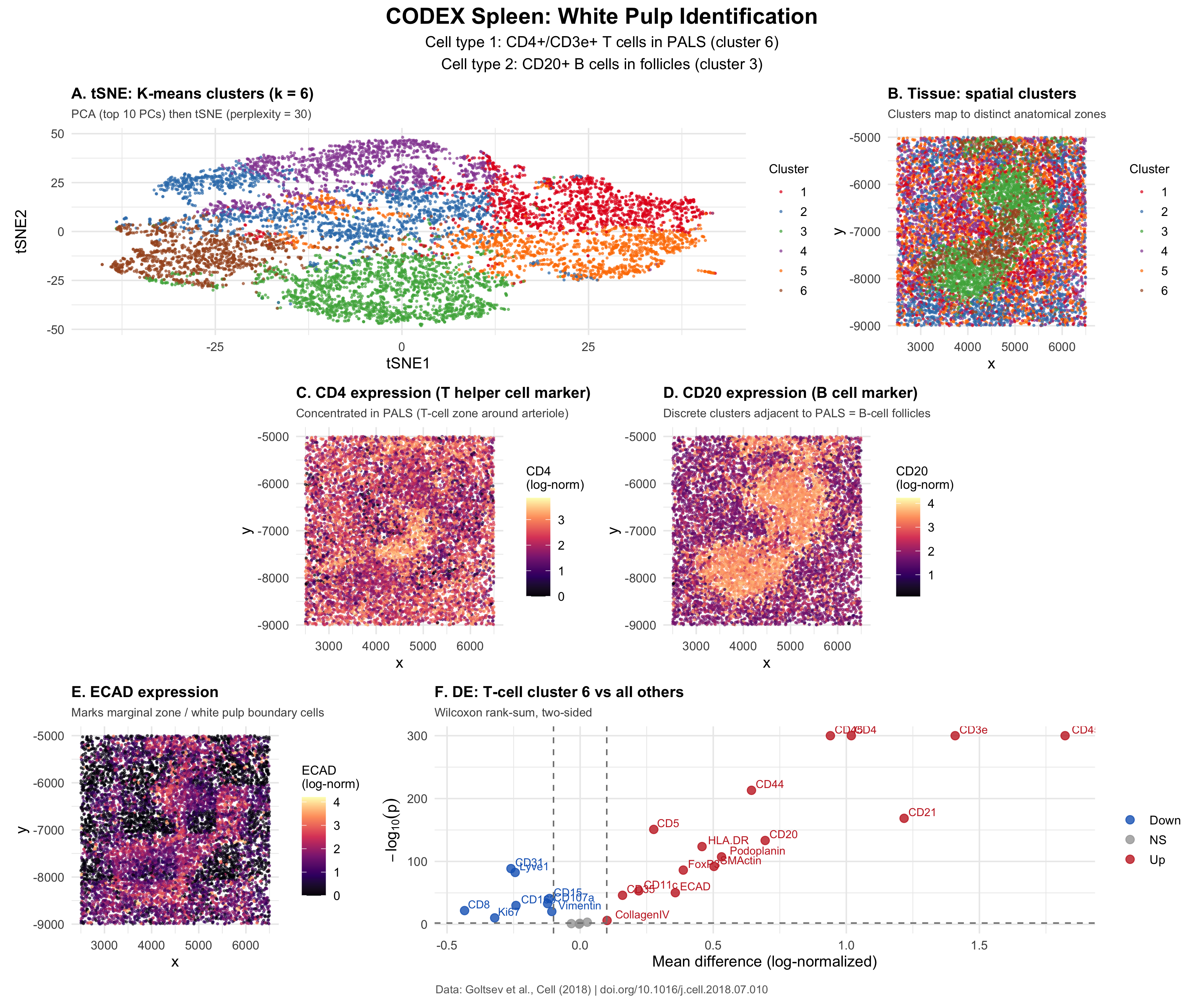
The CODEX spleen dataset contains 28 protein markers for each of 10,000 cells extracted from murine spleen tissue. Then, quality control (removing cells at 1st and 99th percentiles protein expression), normalization (per-cell total-count normalization, log10 transform), PCA, tSNE (perplexity = 30 on top 10 PCs), and k-means clustering (k = 6) were performed. I believe the tissue structure is white pulp based on two cell types that I identified: CD4+ Helper T cells and CD20+ B cells.
Panel A is a tSNE of all cells with color-identified clusters identified through k-means clustering. Panel B takes the clusters and labels them on the original tissue coordinates. Panel C shows CD4 protein expression in the spatial coordinates of the tissue. Panel D shows CD20 protein expression in the spatial coordinates of the tissue. Panel E shows ECAD (E-cadherin) expression in the spatial coordinates of the tissue. Panel F is a volcano plot showing differential expression results for the T-cell cluster (cluster 6) compared to all other cells by using a two-sided Wilcoxon rank-sum test. The identified upregulated proteins are shown in red on the right side while the downregulated proteins are shown in blue on the left side. The x-axis is the mean expression difference and the y-axis is -log10(p-value).
Differential expression analysis (two-sided Wilcoxon rank-sum test) of cluster 6 against all other cells showed upregulation of CD4, CD3e, CD45RO, CD44, CD21, CD5, HLA-DR, and Podoplanin, displayed in Panel F. One of the genes, CD3e, is a part of the TCR complex that is expressed only on T cells (https://doi.org/10.3390/cancers15041012), confirming that cluster 6 contains T cells. Another, CD4, identifies helper T cells instead of cytotoxic T cells. It was also seen that CD8 was downregulated, a symbol of CD4+ helper T cells instead of CD8+ cytotoxic cells, further confirming the CD4 finding. CD45RO is a marker for memory T cells and CD5 is a marker for pan-T-cells, showing that these are memory or activated T cells, rather than naive T cells.
In the tissue spatial plot found in Panel C, CD4 expression is concentrated to specific regions. This region is similar to the periarteriolar lymphoid sheath (PALS). These are T-cell-rich regions that surround the central arteriole in splenic white pulp (https://doi.org/10.1080/01926230600867743). The PALS is a feature of white pulp and contains predominantly CD4+ helper T cells (https://pmc.ncbi.nlm.nih.gov/articles/PMC1828535/).
Cluster 3 shows the highest expression of CD20. This gene is a B lymphocyte surface marker (https://pubmed.ncbi.nlm.nih.gov/14688067/). In the tissue spatial plot found in Panel D, CD20 expression forms discrete, round clusters that are adjacent to the T-cell zone. These clusters correspond to B-cell follicles, the other defining compartment of white pulp. B-cell follicles in the spleen contain naive and memory B cells organized into primary and secondary follicles (https://doi.org/10.1080/01926230600867743).
E-cadherin expression seen in panel E shows cells at the boundary of the white pulp region. In the spleen, ECAD has been associated with marginal zone structural cells that delineate the white pulp from the surrounding red pulp (https://pmc.ncbi.nlm.nih.gov/articles/PMC7112368/). The spatial pattern of E-cadherin shows a boundary-like distribution around the white pulp core. This supports the white pulp interpretation.
The spatial organization that is visible across panels B to E shows a T-cell zone (CD4+/CD3e+) that is flanked by discrete B-cell clusters (CD20+). ECAD can also be seen at the periphery, which are boundary markers. This distribution of cell types (PALS surrounded by B-cell follicles) best represents splenic white pulp over other tissue structures (https://doi.org/10.1080/01926230600867743).
Code
1
2
3
4
5
6
7
8
9
10
11
12
13
14
15
16
17
18
19
20
21
22
23
24
25
26
27
28
29
30
31
32
33
34
35
36
37
38
39
40
41
42
43
44
45
46
47
48
49
50
51
52
53
54
55
56
57
58
59
60
61
62
63
64
65
66
67
68
69
70
71
72
73
74
75
76
77
78
79
80
81
82
83
84
85
86
87
88
89
90
91
92
93
94
95
96
97
98
99
100
101
102
103
104
105
106
107
108
109
110
111
112
113
114
115
116
117
118
119
120
121
122
123
124
125
126
127
128
129
130
131
132
133
134
135
136
137
138
139
140
141
142
143
144
145
146
147
148
149
150
151
152
153
154
155
156
157
158
159
160
161
162
163
164
165
166
167
168
169
170
171
172
173
library(ggplot2)
library(Rtsne)
library(patchwork)

set.seed(42)

## READ IN DATA
setwd("/Users/emmameihofer/Documents/GitHub/genomic-data-visualization-2026")
data <- read.csv("data/codex_spleen2.csv.gz")
pos  <- data[, 2:3]
pexp <- data[, 5:ncol(data)]
rownames(pos) <- rownames(pexp) <- data[, 1]

## QC
totpexp <- rowSums(pexp)
keep <- totpexp > quantile(totpexp, 0.01) & totpexp < quantile(totpexp, 0.99)
cat("Cells before QC:", nrow(pexp), "\n")
cat("Cells after QC: ", sum(keep), "\n")
pos <- pos[keep, ]; pexp <- pexp[keep, ]; totpexp <- totpexp[keep]

## NORMALIZE
mat <- as.matrix(log10(pexp / totpexp * mean(totpexp) + 1))

## PCA
pcs <- prcomp(mat, center = TRUE, scale. = FALSE)

## tSNE
set.seed(42)
emb <- Rtsne(pcs$x[, 1:10], dims = 2, perplexity = 30)$Y
colnames(emb) <- c('tSNE1', 'tSNE2')
rownames(emb) <- rownames(mat)

## K-MEANS (k = 6)
set.seed(42)
clusters <- as.factor(kmeans(pcs$x[, 1:10], centers = 6, nstart = 10)$cluster)
cat("\nCluster sizes:\n"); print(table(clusters))

## IDENTIFY CELL-TYPE CLUSTERS
cluster_means <- sapply(levels(clusters), function(cl)
  colMeans(mat[clusters == cl, ]))

## B-cell cluster: highest CD20
b_cluster <- names(which.max(cluster_means['CD20', ]))

## T-cell cluster: highest CD3e (excluding the B cluster)
t_scores <- cluster_means['CD3e', ]
t_scores[b_cluster] <- -Inf
t_cluster <- names(which.max(t_scores))

cat("\n>>> T-cell cluster:", t_cluster, "\n")
cat(">>> B-cell cluster:", b_cluster, "\n")

## DIFFERENTIAL EXPRESSION — two-sided test
t_cells <- names(clusters)[clusters == t_cluster]
others  <- names(clusters)[clusters != t_cluster]

t_results <- sapply(colnames(mat), function(g)
  wilcox.test(mat[t_cells, g], mat[others, g],
              alternative = 'two.sided')$p.value)
t_fc <- sapply(colnames(mat), function(g)
  mean(mat[t_cells, g]) - mean(mat[others, g]))

cat("\nTop DE in T-cell cluster (two-sided):\n")
print(head(sort(t_results), 8))

## SIX-PANEL FIGURE
df <- data.frame(pos, emb, clusters, mat, check.names = FALSE)

cluster_cols <- c('#e41a1c','#377eb8','#4daf4a','#984ea3','#ff7f00','#a65628')
names(cluster_cols) <- levels(clusters)

base_theme <- theme_minimal(base_size = 11) +
  theme(plot.title    = element_text(face = 'bold', size = 11),
        plot.subtitle = element_text(size = 8.5, color = 'grey30'),
        legend.key.height = unit(0.5, 'cm'),
        legend.title  = element_text(size = 9))

## Panel A: tSNE clusters
pA <- ggplot(df, aes(x = tSNE1, y = tSNE2, col = clusters)) +
  geom_point(size = 0.4, alpha = 0.6) +
  scale_color_manual(values = cluster_cols) +
  labs(title = 'A. tSNE: K-means clusters (k = 6)',
       subtitle = 'PCA (top 10 PCs) then tSNE (perplexity = 30)',
       color = 'Cluster') +
  base_theme

## Panel B: Spatial clusters
pB <- ggplot(df, aes(x = x, y = y, col = clusters)) +
  geom_point(size = 0.4, alpha = 0.6) +
  scale_color_manual(values = cluster_cols) +
  coord_fixed() +
  labs(title = 'B. Tissue: spatial clusters',
       subtitle = 'Clusters map to distinct anatomical zones',
       color = 'Cluster') +
  base_theme

## Panel C: CD4 in tissue
pC <- ggplot(df, aes(x = x, y = y, col = CD4)) +
  geom_point(size = 0.4, alpha = 0.6) +
  scale_color_viridis_c(option = 'magma') +
  coord_fixed() +
  labs(title = 'C. CD4 expression (T helper cell marker)',
       subtitle = 'Concentrated in PALS (T-cell zone around arteriole)',
       color = 'CD4\n(log-norm)') +
  base_theme

## Panel D: CD20 in tissue
pD <- ggplot(df, aes(x = x, y = y, col = CD20)) +
  geom_point(size = 0.4, alpha = 0.6) +
  scale_color_viridis_c(option = 'magma') +
  coord_fixed() +
  labs(title = 'D. CD20 expression (B cell marker)',
       subtitle = 'Discrete clusters adjacent to PALS = B-cell follicles',
       color = 'CD20\n(log-norm)') +
  base_theme

## Panel E: ECAD in tissue
pE <- ggplot(df, aes(x = x, y = y, col = ECAD)) +
  geom_point(size = 0.4, alpha = 0.6) +
  scale_color_viridis_c(option = 'magma') +
  coord_fixed() +
  labs(title = 'E. ECAD expression',
       subtitle = 'Marks marginal zone / white pulp boundary cells',
       color = 'ECAD\n(log-norm)') +
  base_theme

## LLM Prompt:  Can you help me show not only the upregulated, but downregulated genes on Panel F
## Panel F: Volcano — two-sided, colored by direction
t_pv <- -log10(pmax(t_results, 1e-300))
vol <- data.frame(fc = t_fc, pv = t_pv, protein = names(t_fc))
vol$category <- ifelse(vol$fc > 0.1 & vol$pv > 2, 'up',
                ifelse(vol$fc < -0.1 & vol$pv > 2, 'down', 'ns'))

pF <- ggplot(vol, aes(x = fc, y = pv, col = category)) +
  geom_point(size = 2.5, alpha = 0.8) +
  geom_text(data = vol[vol$category != 'ns', ],
            aes(label = protein),
            size = 2.8, hjust = -0.15, vjust = -0.3, show.legend = FALSE) +
  scale_color_manual(values = c('down' = '#1565c0', 'ns' = 'grey65', 'up' = '#c62828'),
                     labels = c('Down', 'NS', 'Up'),
                     name = '') +
  geom_hline(yintercept = 2, linetype = 'dashed', color = 'grey50') +
  geom_vline(xintercept = c(-0.1, 0.1), linetype = 'dashed', color = 'grey50') +
  labs(title = paste0('F. DE: T-cell cluster ', t_cluster, ' vs all others'),
       subtitle = 'Wilcoxon rank-sum, two-sided',
       x = 'Mean difference (log-normalized)',
       y = expression(-log[10](p))) +
  base_theme

## ASSEMBLE AND SAVE
final <- (pA + pB) / (pC + pD) / (pE + pF) +
  plot_annotation(
    title   = 'CODEX Spleen: White Pulp Identification',
    subtitle = paste0(
      'Cell type 1: CD4+/CD3e+ T cells in PALS (cluster ', t_cluster, ')\n',
      'Cell type 2: CD20+ B cells in follicles (cluster ', b_cluster, ')'),
    caption = 'Data: Goltsev et al., Cell (2018) | doi.org/10.1016/j.cell.2018.07.010',
    theme   = theme(
      plot.title    = element_text(face = 'bold', size = 16, hjust = 0.5),
      plot.subtitle = element_text(size = 11, hjust = 0.5, lineheight = 1.2),
      plot.caption  = element_text(size = 8, color = 'grey40', hjust = 0.5)
    )
  )

png('codex_whitepulp_analysis.png', width = 14, height = 15,
    units = 'in', res = 250)
print(final)
dev.off()

cat("\n✓ Figure saved to codex_whitepulp_analysis.png\n")

ggsave('hw5_figure.png', final, width = 12, height = 10, dpi = 300, bg = "white")
ggsave("~/Downloads/emeihof1_HW5.png", final, width = 12, height = 10, dpi = 300, bg = "white")