HW5: Identifying White Pulp and Red Pulp in CODEX Data

Description

The White Pulp (Clusters 1 & 2):

The literature describes the white pulp as lymphatic tissue organized into specific zones that help initiate an adaptive immune response. The germinal center, which is innermost area of the white pulp, contains B-cells, and the surrounding marginal zone contains T-cells [2]

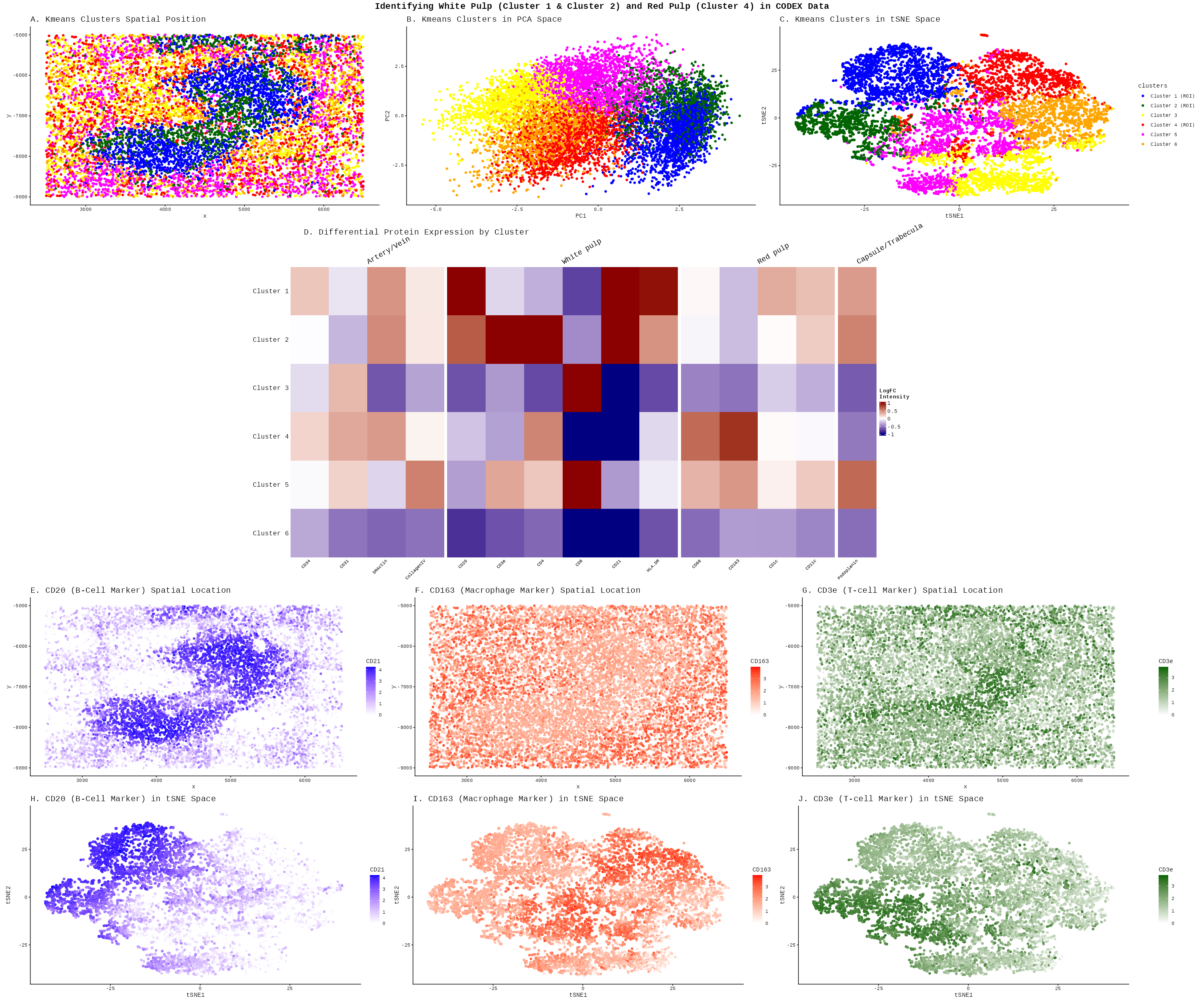
• Spatial Architecture (Panel A): Clusters 1 (Blue) and 2 (Green) form dense, organized nodules. This mirrors the description of “lymphatic tissue surrounding a central arteriole.”

• B-Cell Germinal Centers: Panel E and Pandel H (CD20/B-cell marker) shows high intensity in cluster 1 and is not as intense in the other clusters. In my Heatmap (Panel D), Cluster 1 shows high expression for markers for B-Cells (CD20 and CD20), likely representing these germinal centers.

• T-Cell Zones (periarteriolar lymphoid sheath/Marginal Zone): Panel G (CD3e/T-cell marker) shows a surrounding layer around the B-cell cores. In my Heatmap, Cluster 2 expresses T-cell markers strongly (CD3e and CD4), corresponding to the PALS and marginal zones described in the literature [1, 2].

The Red Pulp (Cluster 4):

The red pulp is a surrounding area containing venous sinuses and macrophages for blood filtration.

• Spatial Distribution: In Panel A, Cluster 4 (Orange) acts as the “background” or interstitial space that surrounds the white pulp nodules, consistent with the description that “white pulp throughout the spleen is surrounded by red pulp.”

• Macrophage Filtering: Panel F nd Panel I shows the CD163 (Macrophage marker). The expression is diffuse and widespread throughout the regions occupied by Cluster 4 and Cluster 5. The macrophage protein expression is lighter in the white pulp area that I defined earlier. This aligns with the red pulp’s role in containing macrophages that “filter abnormal or aging erythrocytes” [1]. Heatmap Evidence: In Panel D, Cluster 4 shows distinct enrichment for markers labeled under the ‘Red pulp’ section, specially macrophage markers (CD68, CD163) [1].

• Cluster 4 also contains SMA and CD34 because those markers define the blood vessels (arteries/veins) and structural bands (trabeculae) that feed the organ. In the white pulp, we only have lymphocytes, but in Cluster 4, the macrophages are permanently attached to the vessels and muscle. My kmeans groups them in cluster 4 because these elements form a single functonal and spatial unit within the red pulp. As noted in the literature, macrophages reside within the splenic cords and sinuses, so their protein signatures are overlapping rather than distinct. While the algorithm easily separated the lymphoid cells of the white pulp, the structural ‘scaffolding’ and the ‘resident’ macrophages of the red pulp might be too physically intertwined at this resolution to be split into separate clusters [1, 2].

References:

[1] (2004). CLUSTER OF DIFFERENTIATION (CD) ANTIGENS. Immunology Guidebook, 47–124. https://doi.org/10.1016/B978-012198382-6/50027-3

[2] Kapila V, Wehrle CJ, Tuma F. Physiology, Spleen. [Updated 2023 May 1]. In: StatPearls [Internet]. Treasure Island (FL): StatPearls Publishing; 2025 Jan-. Available from: https://www.ncbi.nlm.nih.gov/books/NBK537307/

Code

install.packages("BiocManager")
BiocManager::install("ComplexHeatmap")
install.packages('circlize')
install.packages('patchwork')
install.packages('Rtsne')
library(patchwork)
library(ComplexHeatmap)
library(circlize)
library(ggplot2)
library(Rtsne)

set.seed(123)
data <- read.csv('C:/users/lilli/Downloads/codex_spleen2.csv.gz')

#protein data
pexp <- data[, 5:ncol(data)]
#rownames are the cells
rownames(pexp) <- data[,1]
#positions of the data
pos <- data[, c('x', 'y')]
area <- data[, 4]

#normalize protein intensity expression
total_pexp <- rowSums(pexp)
norm_pexp <- (pexp/total_pexp) * mean(total_pexp)
mat <- log10(norm_pexp + 1)

#checking the total withiness to see what K to use
ks <- 1:15
totws <- sapply(ks, function(k) {clus <- kmeans(mat, centers = k)
                                return(clus$tot.withinss)})
totws_df <- data.frame(k = ks, totw = totws)
# elbow plot
ggplot(totws_df, aes(x = k, y = totw)) +
  geom_point() +
  theme_classic() +
  labs(x = 'K', y = 'Total Withiness')
#looks like 6 clusters is enough

#performing kmeans on the full protein expression data
kmeans_result <- kmeans(mat, centers = 6)

#perform PCA
pcs <- prcomp(mat, center=TRUE, scale=FALSE)

variances <- pcs$sdev^2
prop_variance <- variances / sum(variances)
plot(prop_variance)
#looks like I only need to use 10 pcs

clusters <- as.factor(kmeans_result$cluster)

tsne <- Rtsne(pcs$x[, 1:10], dims = 2, perplexity =30)

df <- data.frame(pos, mat, pcs$x, clusters, tsne$Y)

#to keep consistant coloring 
cluster_labels <- c('1'='Cluster 1 (ROI)', '2'='Cluster 2 (ROI)', '3'='Cluster 3', '4' = 'Cluster 4 (ROI)', '5' = 'Cluster 5', '6'='Cluster 6')
cluster_colors <- c('Cluster 1 (ROI)'='blue', 'Cluster 2 (ROI)'='darkgreen', 
                    'Cluster 3'='yellow', 'Cluster 4 (ROI)' = 'red', 
                    'Cluster 5' = 'magenta', 'Cluster 6'='orange')

df$clusters <- factor(cluster_labels[as.character(df$clusters)],  levels = cluster_labels)

p1<- ggplot(df, aes(x=x, y=y, color=clusters))+
    geom_point()+
    scale_color_manual(values= cluster_colors)+
    theme_classic()+
    labs(title = 'A. Kmeans Clusters Spatial Position')+
    theme(plot.title = element_text(size = 15))+
    theme(legend.position ='none')
p2<-ggplot(df, aes(x=PC1, y=PC2, color=clusters))+
    geom_point()+
    scale_color_manual(values= cluster_colors)+
    theme_classic()+
    labs(title = 'B. Kmeans Clusters in PCA Space')+
    theme(plot.title = element_text(size = 15))+
    theme(legend.position ='none')
p3<- ggplot(df, aes(x=X1, y=X2, color=clusters))+
    geom_point()+
    scale_color_manual(values= cluster_colors)+
    theme_classic()+
    labs(title = 'C. Kmeans Clusters in tSNE Space', x='tSNE1', y='tSNE2')+
    theme(plot.title = element_text(size = 15))

#differential gene expression
#loop through all clusters
#I am using the code from lecture 6 and code from HW4 and HW3
de_results <- lapply(1:6, function(k) {
  cluster_of_interest <- names(kmeans_result$cluster)[kmeans_result$cluster == k]
  other_cells <- names(kmeans_result$cluster)[kmeans_result$cluster != k]

  p_values <- numeric(ncol(mat))
  logFC <- numeric(ncol(mat))

  for (i in 1:ncol(mat)) {
    group1 <- mat[cluster_of_interest, i]
    group2 <- mat[other_cells, i]

    test <- wilcox.test(group1, group2, alternative = 'greater')
    p_values[i] <- test$p.value
    #log fold change since data is log transformed
    logFC[i] <- mean(group1) - mean(group2)}

  data.frame(cluster=k, protein=colnames(mat), p_value=p_values, logFC=logFC)})

#combine
de_results <- do.call(rbind, de_results)

#significant
sig_results <- de_results[de_results$p_value < 0.05, ]

#https://www.proteinatlas.org/humanproteome/single+cell/tissue+cell+type/Spleen#
#Tablin, F., Chamberlain, J.K., Weiss, L. (2002). The Microanatomy of the Mammalian Spleen. In: Bowdler, A.J. (eds) The Complete Spleen. Humana Press, Totowa, NJ. https://doi.org/10.1007/978-1-59259-124-4_2
protein_groups <-list('Artery/Vein'= c('CD34', 'CD31', 'SMActin', 'CollagenIV'),
                      'White pulp'= c('CD20', 'CD3e', 'CD4', 'CD8', 'CD21', 'HLA.DR'),
                      'Red pulp'= c('CD68', 'CD163', 'CD1c', 'CD11c'),
                      'Capsule/Trabecula'= c('Podoplanin'))

#flatten into ordered vector
all_proteins <- unlist(protein_groups)
col_split <- factor(rep(names(protein_groups), lengths(protein_groups)),
                    levels = names(protein_groups))

lfc_mat <- tapply(de_results$logFC, list(de_results$cluster, de_results$protein), FUN = mean)
rownames(lfc_mat) <- paste0('  Cluster ', 1:6)

#I followed this tutorial: https://biostatsquid.com/heatmaps-with-complexheatmap-r-tutorial/
p4<- Heatmap(lfc_mat[, all_proteins],
        name = 'LogFC \nIntensity',
        col = colorRamp2(c(-1, 0, 1), c('navy', 'white', 'darkred')),
#I asked AI: I want a heatmap with column grouping brackets at the top.
#Can you add that to my current heatmap?
        column_split = col_split,
        column_title_rot = 30,
        column_gap = unit(2, 'mm'),
        cluster_columns = FALSE,
        cluster_column_slices = FALSE,
        cluster_rows = FALSE,

        column_names_rot = 45,
        column_names_gp = gpar(fontsize = 8),
        row_names_side = 'left')


p5<-ggplot(df, aes(x=x, y=y, color=CD21))+
    geom_point()+
    scale_color_gradient(low = 'white', high = 'blue')+
    theme_classic()+
    labs(title = 'E. CD20 (B-Cell Marker) Spatial Location')+
    theme(plot.title = element_text(size = 15))

p6<-ggplot(df, aes(x=X1, y=X2, color=CD21))+
    geom_point()+
    scale_color_gradient(low = 'white', high = 'blue')+
    theme_classic()+
    labs(title = 'H. CD20 (B-Cell Marker) in tSNE Space', x='tSNE1', y='tSNE2')+
    theme(plot.title = element_text(size = 15))
  
p7<-ggplot(df, aes(x=x, y=y, color=CD163))+
    geom_point()+
    scale_color_gradient(low = 'white', high = 'red')+
    theme_classic()+
    labs(title = 'F. CD163 (Macrophage Marker) Spatial Location')+
    theme(plot.title = element_text(size = 15))
p8<-ggplot(df, aes(x=X1, y=X2, color=CD163))+
    geom_point()+
    scale_color_gradient(low = 'white', high = 'red')+
    theme_classic()+
    labs(title = 'I. CD163 (Macrophage Marker) in tSNE Space', x='tSNE1', y='tSNE2')+
    theme(plot.title = element_text(size = 15))
p9<- ggplot(df, aes(x=x, y=y, color=CD3e))+
    geom_point()+
    scale_color_gradient(low = 'white', high = 'darkgreen')+
    theme_classic()+
    labs(title = 'G. CD3e (T-cell Marker) Spatial Location')+
    theme(plot.title = element_text(size = 15))
p10<-ggplot(df, aes(x=X1, y=X2, color=CD3e))+
    geom_point()+
    scale_color_gradient(low = 'white', high = 'darkgreen')+
    theme_classic()+
    labs(title = 'J. CD3e (T-cell Marker) in tSNE Space', x='tSNE1', y='tSNE2')+
    theme(plot.title = element_text(size = 15))
  
#I asked AI: How to use patchwork on a non ggplot object?
p4_grob <- grid.grabExpr({draw(p4)
  grid.text('D. Differential Protein Expression by Cluster', 
            x = 0.25, y = 0.98,  
            gp = gpar(fontsize = 15))})
#Ask AI: How to stop labels getting cut off in wrap_elements?
p4_new <- wrap_elements(p4_grob, 
                        clip = FALSE)
combined <- (p1 | p2 | p3) /
            ((plot_spacer() | p4_new | plot_spacer()) +
              plot_layout(widths=c(1,3,1))) /
            (p5 | p7 | p9)/
            (p6 | p8 | p10) +
  plot_layout(heights = c(1, 2, 1, 1)) +
  plot_annotation(title = 'Identifying White Pulp (Cluster 1 & Cluster 2) and Red Pulp (Cluster 4) in CODEX Data',
                  theme = theme(plot.title = element_text(hjust = 0.5, size = 16, face = 'bold')))

ggsave('hw5_llam9.png', combined, width = 30, height = 25, units = 'in', dpi = 200, limitsize = FALSE)