Discussion

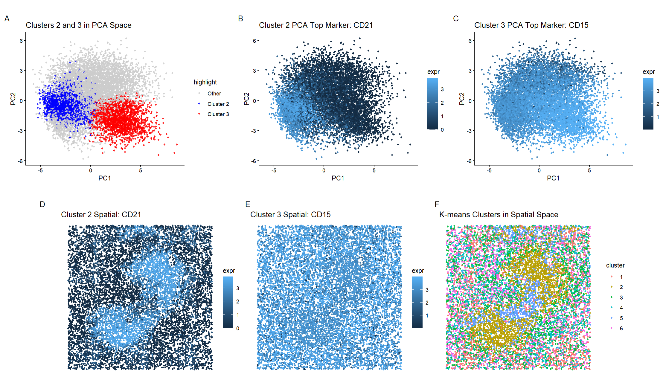
My data visualization has six panels. The first panel shows Cluster 2 and 3 in PCA space, the second panel shows the top marker of Cluster 2 in PCA space, the third panel shows the top marker of Cluster 3 in PCA space, the fourth panel shows the top marker of Cluster 2 in physical space, the fifth panel shows the top marker of Cluster 3 in physical space, and the sixth panel shows the k-means clustering in spatial space.

To determine what tissue structures were represented in the CODEX data, I did the following. I first began with removing data that had very low total intensity. This is data that could negatively impact the PCA and clustering. Then, I scaled and log transformed the data so that the protein signals would be comparable which allowed me to see overall patterns in PCA and k-means. Next, after looking at the elbow plot, I chose to look at the first 10 PCs as after 10, the curve began to flatten. Looking at the k-means scree plot, I chose to split the data into 6 clusters as this is where the scree plot began to flatten out. After choosing the number of clusters, I plotted the clusters in PCA space to determine which clusters were distinct and chose cluster 3 and cluster 6. I then used the Wilcoxon test to determine the differentially expressed genes in each cluster. This is what helped me determine if I did find two distinct cell types.

Looking at Cluster 2, we can see that CD21 has high expression throughout the region which supports that CD21 is a defining marker of this cluster. Looking at Cluster 3, we can see that there is high expression of CD15 throughout most of the cluster. This illustrates that CD15 is a defining marker of Cluster 3.

Cluster 2 Cluster 2 represents a B-cell rich area of the spleen which is found in the white pulp of the spleen. CD21 is highly upregulated on mature B cells and follicular dendritic cells while CD20 (another differentially expressed gene in this cluster) is a definitive marker of mature B cells. HLA-DR (another differentially expressed gene in this cluster) is highly expressed on antigen-presenting cells which is generally found on B cells and dendritic cells. This is supported by the shape that we see in the spatial plot of CD21 as it is mainly concentrated in the middle where the white pulp would be and significantly less expressed outside of this area (where the red pulp and other structures would be).

Cluster 3 Based on literature review, Cluster 3 has a strong upregulation of CD15 alongside increased expression of CD45RO and Ki6. CD15 is a granulocyte marker that is associated with neutrophils. Although CD45RO (a memory T-cell marker) is present, the expression of this marker is weaker than CD15 which means that lymphocytes are not the dominant population. The presence of Ki67 indicates that there is active proliferation which is more consistent with immune activation and inflammatory processes. Therefore, Cluster 3 is most likely a granulocyte-enriched innate immune region which is found in the red pulp of the spleen. This is also reinforced by the spatial plot of CD15 as it is expressed almost evenly throughout with lower expression levels in the middle of the plot (where the white pulp would be).

My literature review demonstrates that I found two different cell types in this data set, B cells and granulocytes. Additionally, based on the combination of the B cells (associated with white pulp) and the granulocyte and endothelial cells I found (associated with red pulp), I would say that the CODEX data most likely represents a section of the spleen that contains both white pulp and some of the surrounding red pulp. This is supported by Panel F where the k-means clustering indicates spatial organization of the spleen with a center that is more homogeneous compared to an outer region that is more heterogeneous. This organization does match the normal spleen structure.

Additionally, as seen in my visualization, specifically in Panel F, we can see that cluster 2 is found primarily in the center and is surrounded by Cluster 3. This further supports the idea that the CODEX data is both white pulp and red pulp as this organization does match the spatial structure of the spleen.

https://pmc.ncbi.nlm.nih.gov/articles/PMC2196095/ https://pmc.ncbi.nlm.nih.gov/articles/PMC3781313/ https://pubmed.ncbi.nlm.nih.gov/15149496/ https://pmc.ncbi.nlm.nih.gov/articles/PMC3781313/

Code

```r

library(ggplot2) library(patchwork)

read in the data

data <- read.csv(“C:/Users/gtbud/Downloads/codex_spleen2.csv.gz”)

separate the data

pos <- data[, 2:3] pexp <- data[, 5:ncol(data)] area <- data[, 4]

rownames(pos) <- data[,1] rownames(pexp) <- data[,1] names(area) <- data[,1]

QC filtering

totpexp <- rowSums(pexp) threshold <- quantile(totpexp, 0.01) keep <- totpexp > threshold

pexp <- pexp[keep, ] pos <- pos[keep, ] area <- area[keep]

normalizing and log transform

pexp_norm <- pexp / rowSums(pexp) pexp_norm <- pexp_norm * 10000 pexp_log <- log10(pexp_norm + 1)

PCA

pcs <- prcomp(pexp_log, scale. = TRUE) X <- pcs$x[, 1:10]

k-means clustering

set.seed(1) k <- 6 kmeans_res <- kmeans(X, centers = k, nstart = 20) clusters <- kmeans_res$cluster names(clusters) <- rownames(X)

PCA dataframe

pc_df <- data.frame( PC1 = X[,1], PC2 = X[,2], cluster = factor(clusters) ) rownames(pc_df) <- rownames(X)

spatial dataframe

space_df <- data.frame(pos) rownames(space_df) <- rownames(pos)

differential protein analysis

mat <- pexp_log clusters_of_interest <- c(2, 3) top10_list <- list()

for(cluster_of_interest in clusters_of_interest){

in_cells <- names(clusters)[clusters == cluster_of_interest] out_cells <- names(clusters)[clusters != cluster_of_interest]

mat_in <- mat[in_cells, , drop = FALSE] mat_out <- mat[out_cells, , drop = FALSE]

mean_in <- colMeans(mat_in) mean_out <- colMeans(mat_out) logFC <- mean_in - mean_out

genes <- colnames(mat) pval <- sapply(genes, function(g) { wilcox.test(mat_in[, g], mat_out[, g])$p.value })

de <- data.frame( protein = genes, logFC = logFC, pval = pval )

de$padj <- p.adjust(de$pval, method = “BH”) de <- de[order(-de$logFC, de$padj), ]

top10 <- de %>% filter(logFC > 0) %>% slice_max(order_by = logFC, n = 10)

top10_list[[paste0(“Cluster”, cluster_of_interest)]] <- top10

cat(“\nTop 10 proteins for Cluster”, cluster_of_interest, “:\n”) print(top10$protein) }

top markers

top_gene_c2 <- top10_list[[“Cluster2”]]$protein[1] top_gene_c3 <- top10_list[[“Cluster3”]]$protein[1]

making the visualization

pc_df$highlight <- “Other” pc_df$highlight[pc_df$cluster == 2] <- “Cluster 2” pc_df$highlight[pc_df$cluster == 3] <- “Cluster 3”

pc_df$highlight <- factor(pc_df$highlight, levels = c(“Other”, “Cluster 2”, “Cluster 3”))

p1 <- ggplot(pc_df, aes(PC1, PC2, color = highlight)) + geom_point(size = 1, alpha = 0.8) + scale_color_manual(values = c( “Other” = “grey80”, “Cluster 2” = “blue”, “Cluster 3” = “red” )) + theme_classic() + coord_fixed() + ggtitle(“Clusters 2 and 3 in PCA Space”)

pc_df$expr <- pexp_log[rownames(pc_df), top_gene_c2] p3 <- ggplot(pc_df, aes(PC1, PC2, color = expr)) + geom_point(size = 1) + theme_classic() + coord_fixed() + ggtitle(paste(“Cluster 2 PCA Top Marker:”, top_gene_c2))

pc_df$expr <- pexp_log[rownames(pc_df), top_gene_c3] p4 <- ggplot(pc_df, aes(PC1, PC2, color = expr)) + geom_point(size = 1) + theme_classic() + coord_fixed() + ggtitle(paste(“Cluster 3 PCA Top Marker:”, top_gene_c3))

space_df$expr <- pexp_log[rownames(space_df), top_gene_c2] p5 <- ggplot(space_df, aes(x = x, y = y, color = expr)) + geom_point(size = 1) + coord_fixed() + theme_void() + ggtitle(paste(“Cluster 2 Spatial:”, top_gene_c2))

space_df$expr <- pexp_log[rownames(space_df), top_gene_c3] p6 <- ggplot(space_df, aes(x = x, y = y, color = expr)) + geom_point(size = 1) + coord_fixed() + theme_void() + ggtitle(paste(“Cluster 3 Spatial:”, top_gene_c3))

space_df$cluster <- factor(clusters[rownames(space_df)])

p7 <- ggplot(space_df, aes(x = x, y = y, color = cluster)) + geom_point(size = 1, alpha = 0.9) + coord_fixed() + theme_void() + ggtitle(“K-means Clusters in Spatial Space”)

final_plot <- (p1 | p3 | p4) / (p5 | p6 | p7) + plot_annotation(tag_levels = “A”) & theme(plot.margin = margin(5,5,5,5))

final_plot

The beginning code was done in class with Prof. Fan.

Most of the code was repurposed from HW3 and HW4

AI was used to construct the for loop (How do I go through and find the genes in my cluster of interest?) and for R syntax

AI was also used to figure out how to format the plots (How do I make sure that all my plots are the same size and things don’t get compressed?)