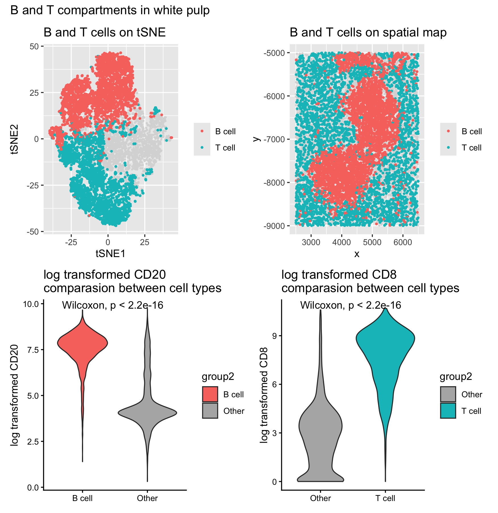
B and T compartments in white pulp

I checked total protein signal and its relationship with cell area, then log-transformed the protein intensities (log1p), ran PCA, embedded cells with tSNE using the top PCs, and applied k-means clustering (k=7 based on the elbow plot). After clustering, I used marker proteins to interpret at two immune cell types and then checked where those cells localize in the tissue.
To interpret the clusters, I used CD20 as a B cell marker and CD8 as a T cell marker. Clusters 1/4/6 are CD20 high and clusters 5/7 are CD8 high, and these two groups do not overlap (which is expected since they represent different lymphocyte lineages). When I highlight these clusters on both the tSNE and the spatial (x,y) map, the B and T cells form clear immune compartments rather than being randomly scattered. That compartmentalized pattern is most consistent with white pulp, which is the organized lymphoid region of the spleen.
This interpretation is supported by work: Pack, Maggi et al. “DEC-205/CD205+ dendritic cells are abundant in the white pulp of the human spleen, including the border region between the red and white pulp.” Immunology vol. 123,3 (2008): 438-46. doi:10.1111/j.1365-2567.2007.02710.x
Finally, I quantified the marker separation using Wilcoxon tests: CD20 is significantly higher in the “B cell” group versus other cells, and CD8 is significantly higher in the “T cell” group versus other cells (shown on the violin plots). Together, the marker enrichment + spatial compartment pattern supports calling this tissue structure white pulp.
I used AI to proofread and refine my text description (prompt“Please proofread and refine my description in my tone”)
1
2
3
4
5
6
7
8
9
10
11
12
13
14
15
16
17
18
19
20
21
22
23
24
25
26
27
28
29
30
31
32
33
34
35
36
37
38
39
40
41
42
43
44
45
46
47
48
49
50
51
52
53
54
55
56
57
58
59
60
61
62
63
64
65
66
67
68
69
70
71
72
73
74
75
76
77
78
79
80
81
82
83
84
85
86
87
88
89
90
91
92
93
94
95
96
97
98
99
100
101
102
103
104
105
106
107
108
109
110
111
112
113
114
115
116
117
118
119
120
121
122
123
124
125
126
127
128
129
130
131
#hw5
library(ggplot2)
library(dplyr)
library(ggpubr)
library(patchwork)

setwd("/Users/tiya/Desktop/BME\ program\ info/Spring\ 2026/gemonic_data_visal/")
data <- read.csv('data/codex_spleen2.csv.gz')

data[1:8,1:8] #X: cell name protein, x,y space, area, intensity reads

dim(data)
pos <- data[, 2:3] #position information
head(pos)

pexp <- data[, 5:ncol(data)] #protein reads data
head(pexp)
rownames(pos) <- rownames(pexp) <- data[,1]

area <- data[, 4] #area data
names(area) <- data[,1]
head(area)


df = data.frame(area, totpexp = rowSums(pexp))
ggplot(df, aes(x = 1, y = log10(totpexp))) + geom_violin()
ggplot(df, aes(x = 1, y = totpexp)) + geom_violin()
ggplot(df, aes(x = area, y = totpexp)) +
  geom_point() +
  geom_smooth(method = "lm") #seem sno corrolation

#normalization on pexp itself
pexp_log <- log1p(pexp)

# PCA
pcs <- prcomp(pexp_log)
df <- data.frame(pcs$x, pos)
plot(pcs$sdev[1:30])
ggplot(df, aes(x=x, y=y, col=PC1)) + geom_point(cex=0.5)
pc = 10

#tSNE
set.seed(2026219)
tsne = Rtsne::Rtsne(pcs$x[, 1:pc], dims = 2, perplexity = 30)

emb = as.data.frame(tsne$Y)

# kmeans
var = numeric(20)
for (k in 1:20) {
  km_result = kmeans(pcs$x[, 1:pc], centers = k)
  var[k] <- km_result$tot.withinss
}

plot(1:20, var, type = "b",
     xlab = "Number of Clusters (k)",
     ylab = "Within-cluster variance",
     main = "Elbow Method")

clusters = as.factor(kmeans(pcs$x[,1:pc], centers=7)$cluster)
df <- data.frame(pcs$x[, 1:3], pos, emb, clusters)
df = cbind(df, area, pexp_log)

#I plan to use CD20 as a B cell marker and CD8 as a T cell marker to find White pulp
#Pack, Maggi et al. “DEC-205/CD205+ dendritic cells are abundant in the white pulp of the human spleen, including the border region between the red and white pulp.” Immunology vol. 123,3 (2008): 438-46. doi:10.1111/j.1365-2567.2007.02710.x

#plotting
ggplot(df, aes(x = x, y = y, color = clusters)) +
  geom_point(cex = 0.5) #spatial plot
ggplot(df, aes(x = V1, y = V2, color = clusters)) +
  geom_point(cex = 0.5) #tSNE plot

ggplot(df, aes(x = x, y = y, color = CD20)) +
  geom_point(cex = 0.5)
ggplot(df, aes(y = CD8, x = clusters)) +
  geom_violin()

b_clust <- as.character(c(1,4,6))
t_clust <- as.character(c(5,7))

df <- df %>%
  mutate(
    hl = case_when(
      clusters %in% b_clust ~ "B cell",
      clusters %in% t_clust ~ "T cell",
      TRUE ~ "Other"
    )
  )
p1 = ggplot(df, aes(x = V1, y = V2)) +
  geom_point(data = df %>% filter(hl == "Other"),
             color = "grey85", size = 0.4) +
  geom_point(data = df %>% filter(hl != "Other"),
             aes(color = hl), size = 0.7) +
  labs(x = "tSNE1", y = "tSNE2", color = NULL) +
  labs(title = "B and T cells on tSNE")

p2 = ggplot(df, aes(x = x, y = y)) +
  geom_point(data = df %>% filter(hl == "Other"),
             color = "grey85", size = 0.4) +
  geom_point(data = df %>% filter(hl != "Other"),
             aes(color = hl), size = 0.7) +
  labs(x = "x", y = "y", color = NULL) +
  labs(title = "B and T cells on spatial map")

df_B <- df %>%
  mutate(group2 = ifelse(hl == "B cell", "B cell", "Other"))

p3 = ggplot(df_B, aes(x = group2, y = CD20, fill = group2)) +
  geom_violin(trim = TRUE) +
  stat_compare_means(method = "wilcox.test") +
  scale_fill_manual(values = c("B cell" = "#F8766D", "Other" = "grey70")) +
  theme_classic() +
  labs(x = NULL, y = "log transformed CD20") +
  labs(title = "log transformed CD20\ncomparasion between cell types")

df_T <- df %>%
  mutate(group2 = ifelse(hl == "T cell", "T cell", "Other"))

p4 = ggplot(df_T, aes(x = group2, y = CD8, fill = group2)) +
  geom_violin(trim = TRUE) +
  stat_compare_means(method = "wilcox.test") +
  scale_fill_manual(values = c("T cell" = "#00BFC4", "Other" = "grey70")) +
  theme_classic() +
  labs(x = NULL, y = "log transformed CD8") +
  labs(title = "log transformed CD8\ncomparasion between cell types")

((p1 | p2) / (p3 | p4)) +
  plot_annotation(
    title = "B and T compartments in white pulp"
  )